Mathematics behind control

If you’re eager to push yourself a little further, you may like to work through this Step. If you do find this a bit too challenging you can always return to this at a later date. Just remember to mark this Step complete before you move to the next.

This Step explains the basic mathematics associated with motors and their controls, justifying why, for instance, when simple control is used the actual speed is less than that desired.

With no control, the motor speed varies due to hills and friction. With simple proportional control (and lower gain) the motor speed is less affected by hills/friction but the speed is lower than that desired.

With better proportional control (higher gain) the speed is even less affected, and closer to what is desired.

With proportional plus integral control the speed is as desired and (in the simplified simulation) unaffected by the hills and friction. Let’s do some calculations to confirm the simulation.

Automatic control of motor

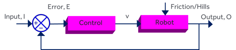
Figure 1: Diagram illustrating automatic motor control (click to expand) © University of Reading

Reminder: this block diagram illustrates what is happening, in terms of the output speed O, the voltage applied to the motor V, K a constant associated with the motor and D which represents the hills/friction

 O = V * K - D 

For control, we also have the desired input, I. We compute the error E and the voltage V by:

 E = I - O and V = calculation based on E

Numbers for no control

We will put some numbers in to illustrate what is happening. For our motor:

 K = 0.125

Suppose we want the desired speed to be 3, then we set V to 24. So if there’s no friction or hills:

 O = 24 * 0.125 = 3

But suppose friction and hills mean D = 0.5 then:

 O = 24 * 0.124 - 0.5 = 2.5

The output speed is much less than we want.

Proportional control, C = 72

Let’s first investigate so called Proportional control, where the controller output is the error multiplied by a constant (it is proportional to the error).
Here C is the constant in the controller, sometimes called its gain, which we initially set to 72.
If the desired input speed is 3, then for P control, E is 3 – O and V is E * C, so:

 V = (3 - O) * C = (3 - O) * 72

Hence, if no friction/hills:

 O = 0.125 * V

So:

 O = (3 - O) * 72 * 0.125 = (3 - O) * 9 = 27 - 9 * O

By gathering all terms associated with O on one side of the equation:

 O + 9 * O = 27

Or:

 10 * O = 27

Dividing both sides of the equation by 10 we get:

 O = 2.7

Clearly the speed is less than the desired value of 3

Hills and friction

Let’s again suppose that hills contribute a value of 0.5 so:

 O = 0.125 * V - 0.5

If C = 72, then V = 72 * (3 – O), so:

 O = 0.125 * 72 * (3 - O) - 0.5
 = 27 - 9 * O - 0.5
 = 26.5 - 9 * O

Gathering all the O terms together:

 O + 9 * O = 10 * O = 26.5

Dividing by 10:

 O = 2.65

Comment

With no feedback control, the 0.5 due to hills/friction reduced the speed by 0.5 from 3 to 2.5. With feedback, without hills, the speed was 2.7.

With hills/feedback the speed was reduced by a further 0.05 to 2.65.

The key point is that Feedback Control has reduced the effect of hills/friction by a factor of 10 (from 0.5 to 0.05) and got the speed closer to the desired value. This is why the robot speed changes less than when there’s no control in the simulation.

What happens if C = 792

We will now investigate what happens when the controller gain is increased to 792. Again, we set
I to 3 and D to 0.5

 O = 792 * 0.125 * (3 - O) - 0.5
 = 99 * 3 - 99 * O - 0.5
 = 296.5 - 99 * O

Gathering terms in O

 O + 99 * O = 100 * O = 296.5

So:

 O = 2.965

Comment

Clearly O is much closer to the desired speed of 3 and the effect of the hills/friction value of 0.5 has been reduced to 0.005.

Proportional plus Integral Control

A controller where V = error * C is called proportional control because the controller output is proportional to the error. To ensure there are no errors, we want integral control. Here the controller output is constant only if its input (which is the error) is zero.

In practice we often use a combination: so called Proportional + Integral control. This is shortened to P + I control. Again the speed is constant only if the error is zero. Hence the output speed equals the desired speed and the hills and friction have no noticeable effect. The so called Advanced Control in the exercise Command the Robot, in Step 3.18, is in fact P + I control. ERIC uses P + I speed control.

It should be noted that in reality, there are some further complications, but that is beyond the scope of the course.