
Big Electricity Energy data
Introduction
By now, we assume that you have a user account to run this example in RStudio on the HPC cluster of the University of Ljubljana.
Load the following libraries:
# perform statistical analysis in R via Hadoop MapReduce functionality on a Hadoop cluster
install.packages("rmr2")
library(rmr2)
# to connect and manipulate stored in HDFS from within R
install.packages("rhdfs")
library(rhdfs)
# to initialise hdfs
hdfs.init()
# dealing with dates
install.packages("lubridate")
library(lubridate)
# tidying and manipulation of data
install.packages("dplyr")
library(dplyr)
install.packages("tidyr")
library(tidyr)
# for plotting
install.packages("ggplot2")
library(ggplot2)
Dataset
A company which sells electricity to its customers has provided a dataset. The dataset is a 15 mins Electricity Consumption data spanning one year for 85 end-users. The dataset also contains Calendar and Weather information.
The file has already been made available on HDFS.
Checking the HDFS files
Check if the ‘electricity-energy.txt’ file of size 454 MB is present in HDFS by running the following command:
hdfs.ls('/')
Note: The file is not a big data file. It can be easily processed on a single processor. The following MapReduce functionality is for demonstration purpose.
Pre-processing
In the first MapReduce job, the script will:
-
- Change the header of columns.
-
- Convert the datatype of columns.
-
- Derive columns Date_Num and Time_Num.
Note: Time_Num can be easily converted to numeric data type using this simple R command:
Z[, "Time_Num"] <- as.numeric(as.factor(Z[, "TimeOfConsumption"]))

head(Z[, c("TimeOfConsumption", "Time_Num")], n=5)
 TimeOfConsumption Time_Num
1 000000 1
2 001500 2
3 003000 3
4 004500 4
5 010000 5
But as we are using MapReduce approach, Mapper may assign the same numeric value to different time intervals depending on the starting value in “TimeOfConsumption” column in input split data assigned to available data nodes. For example, like this:
 Time_Num TimeOfConsumption
1 1 000000
2 1 064500
3 1 011500
4 1 151500
5 2 001500
6 2 070000
7 2 013000
8 2 153000
9 3 003000
10 3 071500
Hence, we will use recode function so every value in time column is assigned only one distinct numeric value.
Next in this script, we will
-
- Select only the required fields.
-
- Aggregate the data of all customers.
Following is the MapReduce script:
mapper1 <- function(., Z){
 colnames(Z) <- c("DateTime", "RegionID", "DateOfConsumption", "TimeOfConsumption", "TBD", "ConsumptionKW_num", "Year", "Month", "Date", "Day", "Weeknum", "HolidayName", "HolidayType", "LongHoliday_flag", "RegionName", "AverageAirPressure_hpa", "Temperature_degC", "RelativeHumidity_perc", "Precipitation_mm", "WindSpeed_mps", "Radiation_Wpm2", "ConsumerID", "Period");
 Z[, "DateTime"] <- ymd_hms(Z[, "DateTime"]);
 Z[, "DateOfConsumption"] <- as.Date(as.character(Z[, "DateOfConsumption"]), '%Y-%m-%d');
 Z[, c("ConsumptionKW_num","AverageAirPressure_hpa", "Temperature_degC", "RelativeHumidity_perc", "Precipitation_mm", "WindSpeed_mps", "Radiation_Wpm2")] <- lapply(Z[, c("ConsumptionKW_num","AverageAirPressure_hpa", "Temperature_degC", "RelativeHumidity_perc", "Precipitation_mm", "WindSpeed_mps", "Radiation_Wpm2")], function(x) as.numeric(as.character(x)));
 Z[, "Day_Num"] <- recode(Z[, "Day"],
 "Monday"=1, "Tuesday"=2, "Wednesday"=3, "Thursday"=4, "Friday"=5, "Saturday"=6, "Sunday"=7);

 Z[, "Time_Num"] <- recode(Z[, "TimeOfConsumption"],
 "000000"=1,"001500"=2,"003000"=3,"004500"=4,"010000"=5,"011500"=6,"013000"=7,"014500"=8,
 "020000"=9,"021500"=10,"023000"=11,"024500"=12,"030000"=13,"031500"=14,"033000"=15,"034500"=16,
 "040000"=17,"041500"=18,"043000"=19,"044500"=20,"050000"=21,"051500"=22,"053000"=23,"054500"=24,
 "060000"=25,"061500"=26,"063000"=27,"064500"=28,"070000"=29,"071500"=30,"073000"=31,"074500"=32,
 "080000"=33,"081500"=34,"083000"=35,"084500"=36,"090000"=37,"091500"=38,"093000"=39,"094500"=40,
 "100000"=41,"101500"=42,"103000"=43,"104500"=44,"110000"=45,"111500"=46,"113000"=47,"114500"=48,
 "120000"=49,"121500"=50,"123000"=51,"124500"=52,"130000"=53,"131500"=54,"133000"=55,"134500"=56,
 "140000"=57,"141500"=58,"143000"=59,"144500"=60,"150000"=61,"151500"=62,"153000"=63,"154500"=64,
 "160000"=65,"161500"=66,"163000"=67,"164500"=68,"170000"=69,"171500"=70,"173000"=71,"174500"=72,
 "180000"=73,"181500"=74,"183000"=75,"184500"=76,"190000"=77,"191500"=78,"193000"=79,"194500"=80,
 "200000"=81,"201500"=82,"203000"=83,"204500"=84,"210000"=85,"211500"=86,"213000"=87,"214500"=88,
 "220000"=89,"221500"=90,"223000"=91,"224500"=92,"230000"=93,"231500"=94,"233000"=95,"234500"=96);

 Y <- Z[, c("DateOfConsumption", "Day_Num", "Time_Num", "ConsumptionKW_num")] %>% as.data.frame();
 key <- paste0(Z$DateOfConsumption, "_", Z$Day_Num, "_", Z$Time_Num);
 val <- Z$ConsumptionKW_num;
 keyval(key, val)
}

mapreduce1 <- from.dfs(
 mapreduce(
 input = '/electricity-energy.txt',
 map = mapper1,
 reduce = function(k, A) {keyval(k,list(Reduce('+', A)))},
 combine = T,
 input.format = make.input.format(format = 'csv', sep=",", stringsAsFactors = F, colClasses = c('character'))
));
We will do the following with the next script:
-
- Bind the key and value columns.
-
- Separate one column to three based on delimiter “_”.
-
- Rename and change the datatypes.
-
- Spread the data on Time_Num and ConsumptionKW_num.
-
- Eliminate NAs.
-
- And store the output in HDFS.
temp <- as.data.frame(cbind(mapreduce1$key, mapreduce1$val))
temp <- separate(data = temp, col = V1, into = c("DateOfConsumption", "Day_Num", "Time_Num"), sep = "_")
colnames(temp)[4] <- "ConsumptionKW_num"
temp[, 2:4] <- lapply(temp[, 2:4], function(x) as.numeric(as.character(x)));
temp <- spread(temp, Time_Num, ConsumptionKW_num)
temp <- temp[rowSums(is.na(temp[,3:98])) == 0,]
input_hdfs2 <- to.dfs(temp)

head(temp[, c("DateOfConsumption", "Day_Num", "1", "2","3", "94", "95", "96")], n=5)
 DateOfConsumption Day_Num 1 2 3 94 95 96
2 2016-10-09 7 7.76 6.80 6.96 12.36 12.60 12.64
3 2016-10-10 1 12.56 13.76 12.08 671.96 666.06 678.08
4 2016-10-11 2 667.22 661.18 636.72 753.88 727.14 704.90
5 2016-10-12 3 735.10 738.30 730.94 602.64 604.26 573.90
6 2016-10-13 4 580.10 592.10 587.48 691.96 658.40 676.82
Day Plots
Following is done in this script:
-
- Declare objects
-
- Calculate length, sum, and the sum of squares
N = 7; # Days in a week
Tn = 96 # Number of measurements in a day
n_vec <- matrix(nrow = 1, ncol = N); # vector of group sizes
sum_mat <- matrix(nrow = N, ncol= Tn); # matrix of group row sums
SS <- matrix(nrow = N, ncol= Tn); # Sum of Squares matrix

mapper2 <- function(., Y){
 for (i in 1:N){
 Yi=as.matrix(subset.matrix(Y[,3:98],Y[,2]==i)); # Matrix for that day
 ni=nrow(Yi); # length of day i
 si=colSums(Yi); # sum of day i for every 15 mins time interval
 SSi=Yi^2 %>% colSums(.); # sum of squares for day i for every 15 mins time interval
 n_vec[i]=ni;
 sum_mat[i,]=si;
 SS[i,]=SSi;
 }
 keyval(1:3,list(n_vec,sum_mat,SS));
}

DayMeanSdPlot <- from.dfs(
 mapreduce(
 input = input_hdfs2,
 map = mapper2,
 reduce = function(k, A) {keyval(k,list(Reduce('+', A)))},
 combine = T
 ))
Standard deviation is calculated using the following formula:
In the following script, we calculate mean±standard deviation for every weekday (for all consumers).
DayMeans <- matrix(nrow=N,ncol=Tn) # matrix containing mean vectors as rows
DaySd <- matrix(nrow = N, ncol= Tn);
DayMinus <- matrix(nrow = N, ncol= Tn);
DayPlus <- matrix(nrow = N, ncol= Tn);

for (i in 1:N){
 DayMeans[i,] <- DayMeanSdPlot$val[[2]][i,]/DayMeanSdPlot$val[[1]][i]
 DaySd[i,] <- sqrt(DayMeanSdPlot$val[[3]][i,]/DayMeanSdPlot$val[[1]][i]-(DayMeans[i,]^2))
 DayMinus[i,] <- DayMeans[i,] - DaySd[i,]
 DayPlus[i,] <- DayMeans[i,] + DaySd[i,]
}

DayMeans <- t(DayMeans) %>% as.data.frame
DayMinus <- t(DayMinus) %>% as.data.frame
DayPlus <- t(DayPlus) %>% as.data.frame
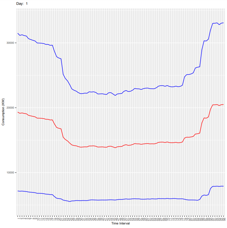
The next script is for generating day plots (replace xyz with username):
pdf("/home/xyz/DayAvgSdPlot.pdf")
for(i in 1:N) {
 print(i)
 print(ggplot()
 + geom_line(data = (DayMeans), aes(x = factor(1:96), y = DayMeans[,i]), color = "red", group = 1)
 + geom_line(data = (DayPlus), aes(x = factor(1:96), y = DayPlus[,i]), color = "blue", group = 1)
 + geom_line(data = (DayMinus), aes(x = factor(1:96), y = DayMinus[,i]), color = "blue", group = 1)
 + xlab('Time Interval')
 + ylab('Consumption in KW')
 + ggtitle(paste("Day: ", i))
 + theme(text = element_text(size=7), axis.text.x = element_text(angle=90, hjust=1))
 + scale_y_continuous("Consumption (KW)", limits=c(min(DayMinus), max(DayPlus)))
 )
}
dev.off()
Below are the output plots:
- Monday
- Tuesday
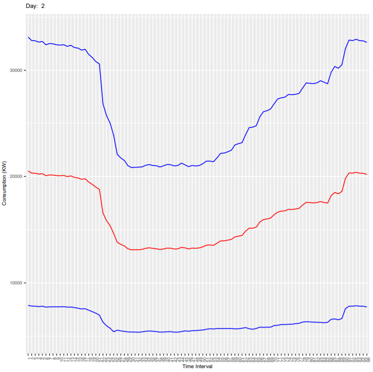
- Wednesday
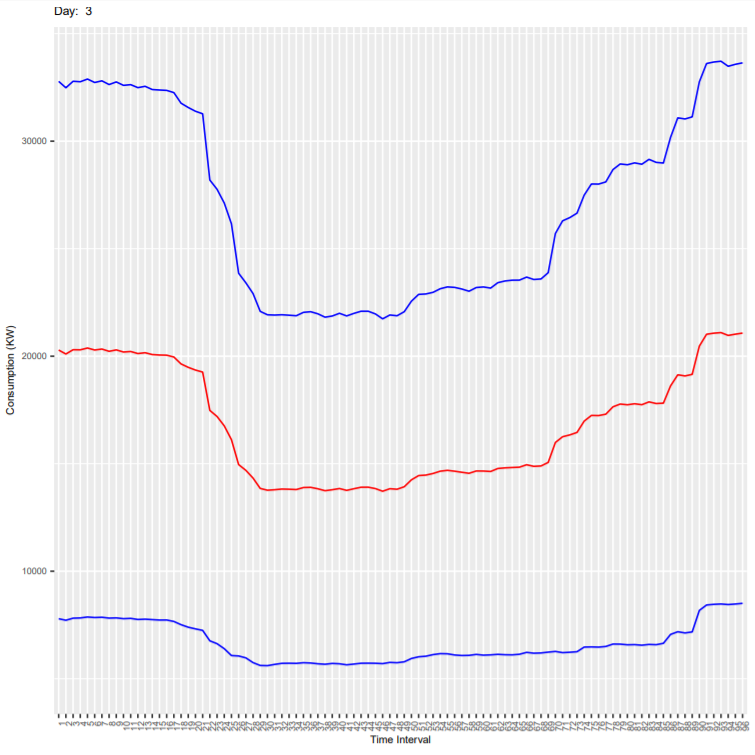
- Thursday
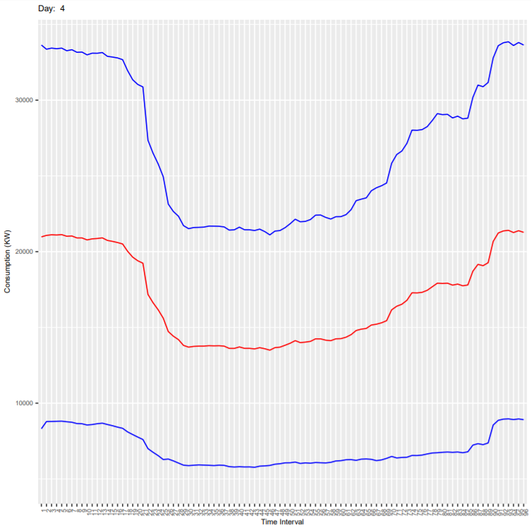
- Friday
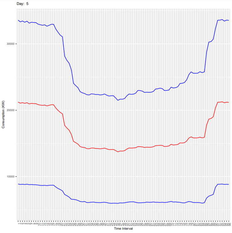
- Saturday
- Sunday
It can be seen that the deviation is more because these plots are for all end-users and every consumer has different consumption habit. As an exercise, you can subset the dataset for one customer (column ConsumerID in the dataset) and generate the plots again. In the new generated plot:
- Check if the deviation is reduced
- Check if the consumption is less on weekends compared to weekdays.
- Check how the consumption varies in every 15 mins during the day.


Reach your personal and professional goals
Unlock access to hundreds of expert online courses and degrees from top universities and educators to gain accredited qualifications and professional CV-building certificates.
Join over 18 million learners to launch, switch or build upon your career, all at your own pace, across a wide range of topic areas.


