Your first model: the mathematics

The model that you have used two steps before depicts the task of finding a supply that is sufficient to satisfy a given demand. In reality, parts of this task have to be done by a market operator who makes dispatch decisions, that is, who decides which power plant runs at which load at which point of time.

Let us have a look at how we describe this in our model. First, the model has four hours ((h=1,…,4)) that are spread over day and night and different seasons. For each of these hours, we have chosen a demand level (d_{h}). Furthermore, each of these hours is characterized by the availability of photovoltaic (PV) and wind power (%), which we denote by (phi_h^{PV}) and (phi_h^{Wind}), respectively. These values show what share of possible production of a unit of PV or wind power is actually achievable at this time of day and this time of year.

In the model, you set capacities of five different technologies ((i=1,…,5)): wind power, PV, coal-fired power plants, gas-fired power plants, and nuclear energy. Let us denote the capacities that you have chosen by (q_{i}^{max}) ((i) being the index that denotes the technology). Furthermore, you have made the decision in which order the controllable technologies are to be used. By assumption, the renewables (PV and wind power) are always used first.

Thus, for each hour (h), we can calculate the supply provided by the renewables as (phi_h^{PV}cdot q_{PV}^{max}+ phi_h^{Wind}cdot q_{Wind}^{max}).

If, for this hour, demand is greater than this renewable supply, the controllable technology that is to be used first (say, coal) is deployed either until demand is met or up to its maximal capacity (q_{Coal}^{max}).

If the maximal capacity is not sufficient to satisfy demand, the controllable technology that you want to use second (say, gas) is used, again either until demand is met or up to its maximal capacity (q_{Gas}^{max}).

Finally, the last controllable technology is used, again either until demand is met or up to its maximal capacity (q_{Nuclear}^{max}).

This is done for all four hours. If demand is exactly met at each hour, then the system is balanced. This can fail for two reasons: first, if total production capacity of the controllable technologies (coal, gas, nuclear) is not sufficient to bridge the gap between demand and renewable supply in this hour. Second, if there is already more renewable supply than demand in this hour.

Let’s use an example with two hours. Assume that demand in hour (h=1) (equal to our model summer day) equals (d_{1} = 17) GW and that PV can produce (phi_1^{PV} = 55)% of its capacity (or 5.5 GW) at this hour and wind (phi_1^{Wind} = 35)% (or 3.5 GW). The second hour (equal to our model winter night) has values of (d_{2} = 14) GW, (phi_2^{PV} = 0)% and (phi_2^{Wind} = 50)% (5 GW). Furthermore, assume that you have chosen to deploy coal before gas before nuclear.

Now consider the following three scenarios (all values in gigawatt (GW)):

^{Click to expand}

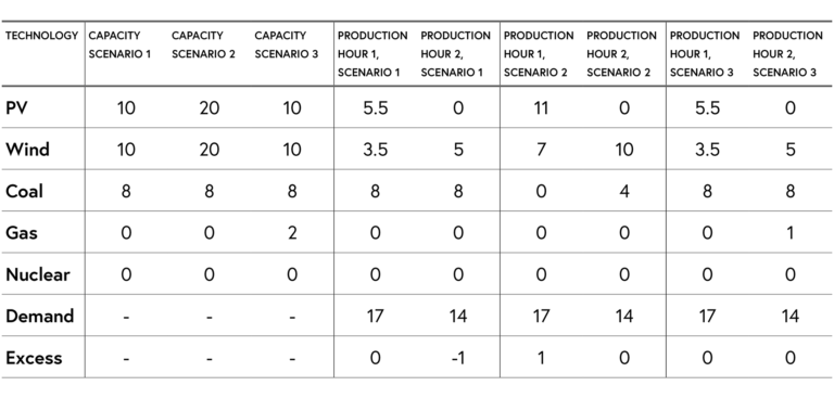
In this example, the capacity in scenario 1 is sufficient for matching demand on a summer day but not on a winter night. In scenario 2, we have increased the capacity of the renewables, but this has led to a situation where there is too much renewable production on the summer day. Finally, in scenario 3, we have used scenario 1 but added gas. In this setting, only renewables and coal are used on the summer day and gas is used to bridge the remaining gap in the winter night. This is the only scenario where the market clears in both hours.

Overall, we can write the model as a constraint for each hour that has to be met:

(1) (phi_1^{PV}cdot q_{PV}^{max}+phi_1^{Wind}cdot q_{Wind}^{max}+phi_{1}^{Coal}cdot q_{Coal}^{max}+phi_{1}^{Gas}cdot q_{Gas}^{max}+phi_{1}^{Nuclear}cdot q_{Nuclear}^{max} = d_{1},)

(2) (phi_2^{PV}cdot q_{PV}^{max}+phi_2^{Wind}cdot q_{Wind}^{max}+phi_{2}^{Coal}cdot q_{Coal}^{max}+phi_{2}^{Gas}cdot q_{Gas}^{max}+phi_{2}^{Nuclear}cdot q_{Nuclear}^{max} = d_{2},)

(3) (phi_3^{PV}cdot q_{PV}^{max}+phi_3^{Wind}cdot q_{Wind}^{max}+phi_{3}^{Coal}cdot q_{Coal}^{max}+phi_{3}^{Gas}cdot q_{Gas}^{max}+phi_{3}^{Nuclear}cdot q_{Nuclear}^{max} = d_{3},)

(4) (phi_4^{PV}cdot q_{PV}^{max}+phi_4^{Wind}cdot q_{Wind}^{max}+phi_{4}^{Coal}cdot q_{Coal}^{max}+phi_{4}^{Gas}cdot q_{Gas}^{max}+phi_{4}^{Nuclear}cdot q_{Nuclear}^{max} = d_{4}.)

In this way of writing the model, the variables (phi_i^{Coal}), (phi_i^{Gas}), (phi_i^{Nuclear}) take values between (0) and (13) and are chosen in the order in which the controllable technologies shall be used to match demand.

This is the complete model that you have used so far. In the following steps, we will add costs and emissions to this model. This will be done in the following way:

Costs will consist of investment costs (c_{i}^{inv}) that are proportional to the capacity for each technology and of variable costs (operating costs, such as fuel costs) (c_{i}^{var}) that are proportional to the actual production in a given hour. For renewables, like PV and wind power, the variable costs are zero. Total costs are simply the sum of investment and variable costs.

Emissions, by which we mean CO₂-emissions, are generated by coal- and gas-fired power plants. Here, we assume that emissions are proportional to production in a given hour. Total emissions are the sum of emissions in all hours.

Finally, let us explain how such a model is fit to actual data, that is, how we calculated the parameters of this model and the following models. Even if we use the model more for illustrative purposes we still aim to make credible assumptions. We need data for the different power plants, for the demand dynamics, and for the renewable availability.

To get variable costs for power plants you will need assumptions on fuel prices, carbon prices, plant efficiency, and emission content of the used fuel. The first two can be obtained from market data; we use average numbers representing European fuel prices in the last decade. Our efficiency values are based on Schröter (2013) as they provide a nice overview on average values. Finally the carbon content can be obtained for example at the EIA webpage. We also use Schröter (2013) as a basis for our investment costs assumptions. As those are given in kilowatt (kW), we need to transfer those into annual fixed costs using classical economic net present value methods to derive meaningful cost levels.

The demand side will be based on the country or region you want to model. We use a fictional country with a peak load of about 20 GW and a total yearly consumption of 150 terawatt hours (TWh) as reference for our model. The respective demand dynamics for summer and winter times are based on the hourly demand levels for European countries as provided by the ENTSO-E. We also assume that the four hours are equally representative for capturing the dynamics of a full year to derive yearly cost numbers.

Finally, the renewable availabilities are derived from historic levels provided by the Renewables.ninja project.

Even if the used model framework, with only four hours and highly aggregated power plant structures, looks rather simplistic it will allow us to derive plenty of meaningful conclusions already as you will see in the next steps.

By using this model as a start you can easily extend the framework by including more hours or more plant types or replacing the dataset with a specific country you are interested in. Starting with a rather simple small scale model first is a good way to ensure your model is doing what you want the model to do. You can always increase the data size later on.

References

Schröder, A. et al. (2013). Data Documentation 68. Current and prospective costs of electricity generation until 2050. Berlin, Deutsches Institut für Wirtschaftsforschung.