Monopoly model: the mathematics II

Now that you have seen your first monopoly model let’s use the setting of our perfect competition example to analyze how such a model can be designed as optimization and as equilibrium model and learn a bit on the economics of monopolies on the way.

The setup is the same with one change: we now assume monopolistic competition.

So instead of many firms, (i), we just have one single firm. This firm does what every firm is doing, it maximizes its profit.

(1)   (max limits_{qgeq 0}⁡ enspace p(q)q-c(q))

But, given that it is the sole supplier on the market, the firm knows that its output decision will have an impact on the market price. That is why, contrary to a perfectly competitive market, the income side is not only price times quantity, (pq), but the price, (p), is now a function of quantity, (q).

Now, how does the firm know how (p) and (q) are related?

Recall the benefit function (B(d)) we used in the perfectly competitive market to model the consumer behaviour. The first order derivative of this function ((frac{∂B}{∂d})) tells us exactly this: how does the willingness of to pay for the product change with a marginal change in consumption ((d)). In other words, you could rewrite the benefit-demand relation as a price-demand relation:

[frac{∂B}{∂d}=p]

For example the demand-price relation we used in the last model exercises was given by:

[d=bar{Q} -η cdot p]

or, rearranging the equation,

(p=frac{d-bar{Q}}{eta }) to be closer to our (p(d)) formulation.

As a last step, you now need to consider that the monopoly is the only supplier in this market. Thus, the normal demand balance is now simply (q = d) making (p(d) = p(q)). Therefore equation (1) is all you need for a monopoly optimization model.

Again, you will need to derive the first order conditions of the model with respect to the choice variable of the monopoly, ((q)), and set it equal to zero:

(2)   (p(q)+frac{∂p(q)}{∂q}q-frac{∂c(q)}{∂q}=0)

Note that the first term in the objective function, (p(q)q), requires you to use the product rule when making the derivation. This is the normal first-order condition of a monopoly.

Let’s switch to the equilibrium formulation. Similar to the perfect competitive version, we have three elements: the monopoly maximizing its profit, consumers maximizing their benefit, and a market that brings the two sides together. Thus, we actually only need to change the firm block and can keep the other elements as before.

Consumers are still described by their zero-profit logic:

(3)   (pgeq frac{∂B}{∂d} bot dgeq 0)

And in the market clearing we just need to replace the output of all firms with the single output of our monopoly:

(4)   (qgeq d bot p geq 0)

The zero-profit condition for the monopoly is a bit more tricky. You can either derive this logic by formulating the maximization problem for the monopoly and make the first order derivation and implement this as the zero-profit condition; so basically what we did above for the optimization model. Or, you know the economic equilibrium condition for the behaviour of a monopoly: marginal revenue equals marginal costs.

In a perfectly competitive world, a firm simply sells its output on the market assuming that its own decision has no impact on the price. Thus, the marginal revenue a competitive firm can obtain is equal to the market price. Consequently the equilibrium condition was: market price equals marginal costs.

But a monopoly knows that its own output decision has an impact on the price. And since it is the only one selling this also has a feedback effect on the total sale revenue. Increasing the output by one unit increases the income by the market price, (p), but as the price declines with higher demand (respective output by the monopolist) the revenue on the total output decreases due to the price reduction. This can be formalized as:

(5)   (frac{∂c(q)}{∂q}geq p+frac{∂p(q)}{∂q}q bot q geq 0)

The left hand side is again the marginal costs, the right hand side is the marginal revenue. A monopoly will produce ((q > 0)) up to the point where its marginal cost level is equal to the additional revenue is can obtain ((frac{∂c(q)}{∂q}= p+frac{∂p(q)}{∂q}q)) defined by the additional income for selling one more unit ((p)) and the reduction in total income on all sold units ((frac{∂p(q)}{∂q}q)). Note that (frac{∂p(q)}{∂q}) is usually negative as the price-demand relation is downward sloping (with a higher demand prices need to decrease and vice versa).

In other words, the optimization and equilibrium model are again providing the same result: a monopoly will produce up to the point where its profit is maximized and this point is defined where the additional revenue it can obtain is equal to the cost it has for this additional output.

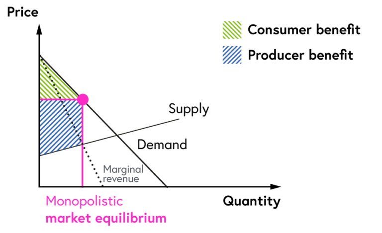
This results in a significant shift between consumer and producer rent, a lower (d) and level at higher market prices, and a total loss in welfare.