Let the computer do the work I: optimizations

Modern computer capacities and advances in modeling software and algorithms make numerical modeling much more accessible than a few decades ago. Nevertheless, basic understandings of the mathematical model structure and its feedback on the design stage are requirements to ensure that the model is not only credible but can also produce meaningful results.

In this step, we will take a short look into some computational aspects that you should keep in mind when designing your model as they often will have a direct impact on if and how your model will solve.

When optimizing models, one of the main choices is between linear or non-linear model designs. A Linear Program (LP) consists of a linear objective function and linear constraints. A common formulation is a cost minimizing LP of the form used in Week 2:

   (min limits_q enspace {Cost}=sum{c_i q_i})  (Cost objective)

 s.t. (q_ileq q_i^{max})  (Production constraints)

   (sum{q_i}geq d)  (Demand constraints)

The advantage of LP formulations is that they can be solved relatively fast even for large scale models. Furthermore, the obtained solution provides a global optimum: either a unique solution, a continuum of equivalent solutions, or no solution. LP models therefore provide a good starting point to get familiar with the problem at hand. Albeit many relations and restrictions in the real world are non-linear oftentimes, they can be reasonably approximated by linear formulations.

Naturally, Non-Linear Programs (NLP) relax the linearity constraints and the functional relations can take on any form. The advantage of NLPs comes with the possibility to remain closer to real world conditions. However, this comes at a price. First, NLPs are harder to solve and will normally need longer to find a solution. Second, most NLP solutions don’t guarantee a global optimum.

Exemplary solution space for a NLP

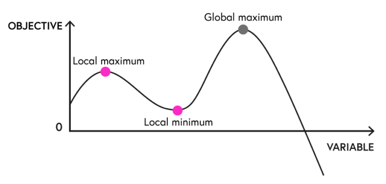
To ensure that a global maximum is reached, further criteria, in addition to the first-order conditions, are needed. There are global solvers that ensure that a solution is a global optima, but the computational effort is much higher than for local solvers. Therefore, most of the time, NLP models will only ensure that a local optima is obtained. From a modeler perspective, this means that one should ensure that the obtained solution is reasonable; for example, by providing starting points via LP approximations of the NLP model.

A special form of NLP models are formulations with quadratic elements. This can either be Quadratic Programs (QP) that have a quadratic term in the objective but only linear constraints (for example typical welfare formulations) or Quadratic Constraints Programs (QCP) in which the side constraints can contain quadratic formulations. Those NLPs are easier to solve and many solvers have special routines for this kind of problem.

A final important form for optimization models are formulations involving integer variables. The most common form of models with integer elements are coded as Mixed-Integer Linear Programs (MILP) that involve both continuous and integer variables while keeping the linearity restrictions. You can also design non-linear formulations with integer elements but the current solver capability for those problems is rather limited. Integer elements are rather common in real life (eg, most commodities are consumed in discrete amounts) but can often be reasonably approximated by continuous formulations for large-scale problems (eg, models with a consumption of 1000.4 units are less of a problem than models with 1.4 units).

A common usage for integer elements are binary variables indicating choices (ie, binary 0-1 variables), like fixed costs added if a production site is constructed. A typical example in electricity markets is power plant status conditions:

   (min_limits {q,s} enspace {Costs}=sum{c_i q_i})  (Cost objective)

 s.t. (s_i q^{min} leq q_i leq s_i {cap}^{max})  (Generation constraint)

   (sum{q_i} geq d)  (Demand constraint)

In case a plant is online ((s = 1)) the output, (q), of a plant (i) has to remain within the generation constraints defined by the lower and upper capacity limits. In case the plant is offline, ((s = 0)), the output is fixed to zero. MILP models are harder to solve than pure LP models but still perform reasonably well, normally obtaining global optimality and they can handle large datasets.

The easy design of optimization problems and the good solver capabilities of modern computers make optimization models a good place to start your endeavour into numerical modeling. You will be able to design large system representations or complex firm optimizations. Even if you want to assess more complex real world challenges, like the oligopoly models we discussed in Week 4, a simple benchmark optimization model representing first-best conditions is often helpful.