We have already seen what a sine wave looks like in time and space – it’s the most basic form of wave.

The Fourier transform lets us to see that same sine wave in a different way. It is a common mathematical tool used by physicists and engineers that changes the representation of spatial or temporal data into frequency data. Among other applications, the Fourier transform is useful when we want to understand how digital sound, such as that from a CD, becomes the analog (continuous) sound that we hear, and whether or not it faithfully reproduces the originally recorded sound.

Sound, of course, is one-dimensional; it changes with time. The Fourier transform can also be used on two-dimensional data such as images. A process very similar to the Fourier transform forms the basis of the JPEG image compression standard widely used on the Internet, for example.

The Continuous Fourier Transform

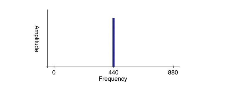
A sine wave consists of only a single frequency, so its representation in the frequency space is very simple: just a single number representing that frequency. For example, the common musical note A above middle C on a piano has a frequency of 440 hertz, so its Fourier transform is just the number 440. We can represent this graphically just as a single vertical bar at the appropriate place:

More complex signals have more complex transforms, but any signal can be broken down into a combination of sine waves and cosine waves (which, of course, are just sine waves shifted by a quarter of a cycle). For our purposes here, we only need to learn about simple signals, but we encourage you to learn as much as you can about the Fourier transform.

The Discrete Fourier Transform

Our abstract example above is the continuous Fourier transform. But normally, when we are working with computers, we have discrete data, a series of samples of the actual signal. We can also calculate the original signal itself using any digital process. Consider the following sequence of bits:

[10001000100010001000100010001000…]

Obviously the pattern repeats itself once every four bits. We would expect that a digital transform of this would give us the number 4.

The result is actually somewhat more complicated than that. Not only does the pattern repeat every four bits, it also repeats every 8 bits, every 12 bits, and so on. Thus, after a little thought, we might instead expect that the transform would give us the sequence (4, 8, 12,…) and this is, in fact, what we get:

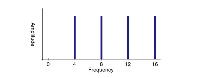
A graph like this is said to be the frequency domain representation of the signal, rather than in the more common temporal domain representation (for a signal that varies in time, like sound) or the spatial domain representation (e.g., for an image).

フーリエ変換

前回までは時間方向と空間方向における最も基本的な波としてsin波について学んできました。

フーリエ変換とは複雑な波を全てsin波で表す形に変換するというものです。データを周期で表すために物理学者やエンジニアに広く一般的に用いられる数学的ツールとして知られています。フーリエ変換を学ぶことで、CDのようなデジタル音声がどのようにして私たちが実際に聞くアナログ（連続）音声になるのかといったことや、録音された音が忠実に再現されているのかどうかといったことを理解できます。

音声は時間と共に変化する1次元の波です。 フーリエ変換は画像などの2次元データに対しても使用できます。 フーリエ変換に非常に類似したプロセスは、例えば、インターネット上で広く使用されているJPEG画像圧縮標準の基礎技術としても用いられています。

連続フーリエ変換

正弦波は単一の周波数のみで構成されているため、周波数空間での表現は非常にシンプルです。例えば、ピアノ上のミドルCの上にある音符A（一般的なピアノでいう所の真ん中のラの音）は440ヘルツの周波数なので、そのフーリエ変換は単に440となります。図形的には440ヘルツの位置に垂直なグラフとして表現できます。

複雑な信号になればなるほどより複雑な変換をしますが、どの信号も正弦波と位相差 2/π の余弦波との組み合わせに分解することができます。この分野を学ぶに当たって単純な信号だけではなく、フーリエ変換についてできるだけ多くのことを学ぶことが大切です。

離散フーリエ変換

これまで説明してきた例は厳密には連続フーリエ変換と呼ばれるものです。しかしながら通常、私たちが使うコンピュータでは実際の信号の一連のサンプルとして、離散データが用いられています。この場合でもデジタルプロセスを使用して元の信号そのものを計算することもできます。次のビット列を考えてみましょう。

[10001000100010001000100010001000…]

パターンが4ビットごとに1回繰り返されていることがわかります。これをデジタル変換しても４という数値を得ることができます。

一見単純見えるかもしれませんが、結果は実際にはそれよりいくらか複雑です。パターンは4ビットごとに繰り返されるだけでなく、8ビットごと、12ビットごとにも繰り返されることになります。したがって変換も 4,8,12,… のシーケンスになると考えられ、実際そうなっています。

このようなグラフは、（音のような時間的に変化する信号の）より一般的な時間領域表現または（例えば上の画像のような）信号の周波数領域表現とも呼ばれています。