Market Equilibrium and Price Controls

In this article, Dr Matthias Dahm takes a closer look at market equilibrium and price controls.

We start by considering a market without price controls. Figure 1 represents a competitive market. The aim of the graphical representation is to explore market exchanges. The horizontal axis indicates the quantity and the vertical axis the price of the good. Figure 1 shows a demand function, which represents consumers in the market. It indicates for each price a quantity demanded. The demand function can be interpreted as the willingness to pay of consumers for the good. The demand function is downward sloping, because of the law of demand: All other factors being equal, as the price of a good increases, the quantity demanded decreases. In other words, the smaller the quantity demanded, the more the willingness to pay for an additional unit of the good. Figure 1 illustrates this, as at Q^L the willingness to pay is P^H, which is higher than P^C at Q^C.

Figure 1

We turn now to the supply side of a market, which represents producers. The supply function indicates for each price a quantity supplied. It can be interpreted as the lowest price that is sufficient for producers to be willing to offer an additional unit in the market. The supply function is upward sloping, because of the law of supply: All other factors being equal, as the price of a good increases, the quantity supplied increases. Again Figure 1 illustrates this, as at Q^L the minimal price is P^L, which is lower than P^C at Q^C.

Once a market has been described using the tools of demand and supply, the next task is to predict the outcome of the market interaction between consumers and producers. Economists think of prices as balancing supply and demand. Markets tend to equilibrium, because prices adjust when for a given price the quantity supplied and the quantity demanded are not compatible. From Figure 1 we see that at the price P^C the quantity supplied equals the quantity demanded. In other words, the market is in equilibrium and the quantity Q^C is exchanged at the price P^C. At other prices supply and demand are not compatible. For instance, at the price P^L the quantity demanded Q^H exceeds the quantity supplied Q^L and so the price tends to rise until P^C is reached.

How should we think of a market equilibrium? Economists think that a market equilibrium is efficient. One way to see why this is the case is to consider a smaller quantity than Q^C, say Q^L. At that quantity the demand function is higher than the supply function, as P^H is larger than P^L. This indicates that the consumers’ willingness to pay for the good exceeds the lowest price necessary for producers to be willing to offer an additional unit in the market. Therefore, from society’s point of view, an additional unit should be exchanged. This argument can be repeated until the quantity Q^C is reached and willingness to pay and minimum price coincide.

Notice that Adam Smith’s metaphor of the ‘invisible hand’ that we encountered in a previous part of the course refers exactly to this property of markets. Even though market participants are not guided by what is best for society, markets lead to efficient situations. This is so, because self-interest leads to a situation in which resources are dedicated to the activities that are most valued, as if guided by an ‘invisible hand’.

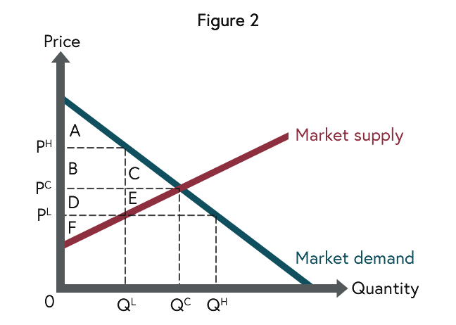Figure 2

Another way to see that the market equilibrium is efficient builds on the concepts of consumer surplus and producer surplus. Both are a measure of welfare of a given market situation. Consumer surplus builds on the demand function, which again is interpreted as indicating the maximal price consumers are willing to pay for the good. So, as we move along the demand curve (from the left to the right) this maximal price decreases until we reach the market price P^C. Thus the area A+B+C represents the value of the good minus the price paid for it, aggregated over the total quantity demanded. This is the consumer surplus generated by the competitive equilibrium. Similarly, producer surplus is measured using the supply function, which is interpreted as indicating the minimal price producers need to produce the good. With this interpretation, the area D+E+F represents the price received minus the production costs of the good, aggregated over the total quantity supplied. This is the producer surplus generated by the competitive equilibrium. The competitive equilibrium is efficient, because it maximises welfare as measured by the sum of consumer and producer surplus. In other words, the area between the demand function and the supply function is maximal: A+B+C+D+E+F. With a smaller quantity than Q^C this area is reduced, as consumer surplus and producer surplus both reduce to a pentagon. With a larger quantity than Q^C this area is also reduced, as a “negative area” is added to A+B+C+D+E+F.

We can now use Figure 2 to understand the effects of price controls. We will focus on price controls that rule out the competitive price P^C. Suppose that the price cannot exceed P^L. Since higher prices are illegal, P^L is a maximum price. We have already seen that in a market the price tends to rise towards the equilibrium price P^C. But now the new price cannot exceed P^L and will hence be exactly P^L. At that price the quantity supplied is Q^L, while the quantity demanded is Q^H. Since Q^L is smaller than Q^H, only Q^L units will be exchanged. Consequently, consumer surplus is A+B+D, while producer surplus is F. This situation is less efficient than the competitive equilibrium, as the area C+E is lost. It is important to notice that this loss represents consumers who cannot buy the good and producers who are not allowed to profitably participate in the market. There is also a distributive effect. Producers are unambiguously worse-off, as the area F is smaller than the area D+E+F. Consumers lose C and gain D, indicating that those consumers who are successful in buying the good benefit from the low price. But as already pointed out, other consumers are not able to buy the good and are also worse-off.

The preceding is the basic logic for why economists tend to argue that price controls are undesirable and the starting point for a deeper analysis of, for example, the long term effects of such an intervention on demand and supply or the emergence of black markets.

The analysis that Matthias has presented in this article is the analysis that many economists use to argue against price controls. However, price controls still exist at some times and in some places around the world. Comment below why this might be the case.