How Do You Calculate VaR?

As we have seen in the previous step, VaR is a quantified measure of risk which is widely used in risk management practice. It’s therefore important to understand how to calculate it.

There are three approaches to calculating VaR:

1. parametric approach
2. historical data approach (or non-parametric approach)
3. Monte-Carlo simulation approach.

Let’s suppose you invest in Firm A’s stock. The question is: what is your maximum possible loss over a given time period for a given confidence interval? For example, you want to know the maximum possible fall in the value of this stock within the next 10 days for a 95% confidence level.

The parametric approach assumes the log of stock prices (and stock returns) follows a normal distribution. There are two parameters describing a normal distribution: the mean and the variance. With this information we can use the probability distribution of stock returns to find out the probability of an event occurring. Formally, VaR can be calculated using the following formula:

[VaR ,= , sigma ,N^{-1}(X)]

Here (X) is the confidence level. What does this mean? If we choose a 95% confidence level, we interpret the VaR we obtain as a measure of the loss we might observe in 5 out of every 100 trading days.

(N)(^{-1}) is the inverse cumulative standard normal distribution. Together with the confidence level, this establishes a cut-off point in the standard normal distribution. We say there is a (1 – (X)) probability of observing points to the left of this cut-off point, and a probability of (X) of observing points to the right of the cut-off point.

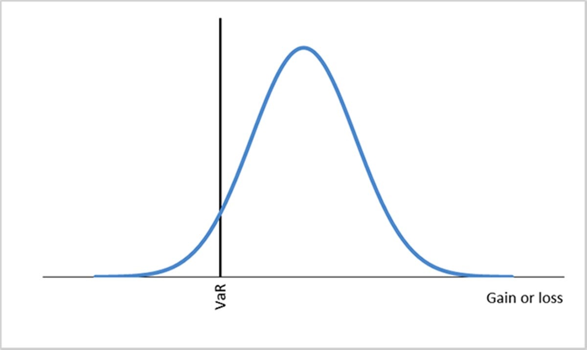
In the standard normal distribution, the 95% cut-off is –1.64 (the 99% cut-off is –2.33). But remember, the standard normal distribution has a standard deviation of 1. To obtain the VaR for our stock, we multiply the cut-off by the standard deviation of the stock return, (sigma). The VaR we obtain is illustrated in the following figure.

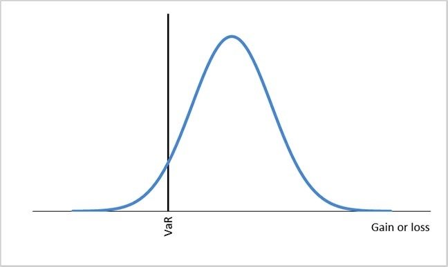
VaR using the normal distribution (Click to expand)

So far we have explained a one-day VaR. If the required time horizon is (T) days, the daily VaR can be translated into the VaR for (T) days using the following formula:

[VaR (T days) =VaR (1 day) times sqrt{T}]

The non-parametric approach does not require us to know the distribution of the stock price. Instead, we collect information on the stock price (and stock return) for a sample of past trading days. We then rank the stock returns from lower to higher returns. VaR reflects potential losses, so our main concern is lower returns. For a 95% confidence level, we find out what is the lowest 5% (1 – 95)% of the historical returns. The value of the return that corresponds to the lowest 5% of the historical returns is then the daily VaR for this stock.

In the Monte Carlo approach, we simulate the performance of a stock (or portfolio of stocks). We repeat the simulation many times to create a distribution of returns, and we use this distribution to compute the measure of value at risk. To conduct the simulation we make assumptions about how the stock prices evolve over time, and we simulate values for the stock prices using a random number generator. This approach provides more flexibility. For example, if we are unhappy about using the normal distribution, we can generate stock prices that follow a distribution with fatter tails.