Simple shape modelling using the multivariate normal distribution

In this article, we will show how we can build a very simple model of hand shapes by modelling the variation in the length and the span of the hand using a bivariate normal distribution. This article serves two purposes: first it illustrates the concepts we introduced in the previous video using a concrete example. Second, it also introduces many key ideas behind statistical shape models. We conclude this article with a note on degenerate normal distributions, which often occur in shape modelling.

A simple shape model

In this first, very simplistic example of a shape model, we assume that the shape of a hand can be characterised by only two measurements: the length (l) and the span (s) of the hand (see Figure 1).

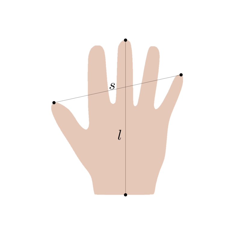^{Figure 1: measurements for the length and the span of a hand shape.}

Our task is to model how these two measurements vary in the family of hand shapes. In this course we always assume that shape variations can be modelled using a normal distribution. Hence, we assume that the random variables (s) and (l) are distributed according to the bivariate normal distribution

$$left( begin{array}{c} l s end{array} right) sim Nleft(left( begin{array}{c} mu_l mu_s end{array} right) , left(begin{array}{cc} sigma_{ll}^2 & sigma_{ls} sigma_{ls} & sigma_{ss}^2 end{array} right) right).$$

In this particular example, this assumption implies that

• it is sensible to think of a mean hand (with average length and average span), around which all plausible hand shapes ‘cluster’;
• it is equally likely for hands to be smaller or larger than this mean;
• we are unlikely to ever observe shapes that are much larger or smaller than the mean.

Thinking about it for a while, we see that these are reasonable assumptions for the length and span of the hand (and indeed for many other anatomical measurements). Our intuition is confirmed by looking at some data. We have compiled a set of measurements of the hand length and span of 72 students. A scatterplot of these measurements is shown in Figure 2. We see that most measurements concentrate around a size of 19 cm for the length and 20 cm for the span.

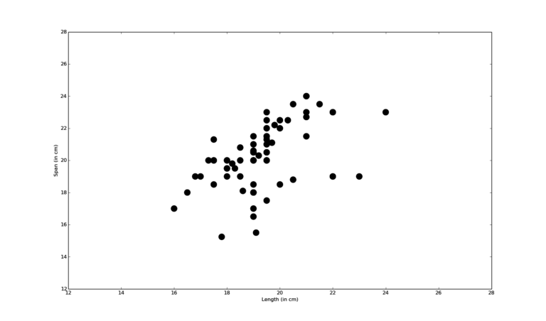^{Figure 2: scatterplot showing measurements of the hand span and length of 72 students.}

Estimating the parameters from data

Once we have chosen the form of the model, we need to define the parameters. While we are in principle free to specify the model parameters based on prior knowledge about the anatomy, a more principled approach is to estimate the parameters from the given data. We use again the measurements shown in Figure 2. Let

$$M = {tilde{x}_1, ldots, tilde{x}_n} = left { left(begin{array}{c}tilde{l}_1 tilde{s}_1 end{array}right), ldots, left(begin{array}{c}tilde{l}_n tilde{s}_n end{array}right) right }$$

denote the set of measurements.

We can estimate the mean and covariance matrix from (M) using the following standard formulas for the sample mean

$$mu = frac{1}{n}sum_{i=1}^n tilde{x}_i$$

and the sample covariance

$$Sigma = frac{1}{n-1} sum_{i=1}^n (tilde{x}_i – mu)(tilde{x}_i – mu)^T.$$

Using the data shown in Figure 2 to estimate these parameters, we obtain the statistical shape model defined by the following bivariate normal distribution:

$$x sim Nleft(left( begin{array}{c} 19.3 20.2 end{array} right) , left(begin{array}{cc}2.1 & 1.4 1.4 & 3.8 end{array} right) right ).$$

Using the model to reason about shapes

We can now use this model for exploring the shape family and reasoning about individual shapes. First, we can directly read off from the distribution that the corresponding marginal distribution for the length alone is (p(l) = N(mu_{l}, sigma_{ll}^2) = N(19.3, 2.1)) and for the span we have (p(s)=N(mu_{s}, sigma_{ss}^2) =N(20.2, 3.8)). Not surprisingly, the variation of the span is larger than the variation in length (this is due to the fact that people spread the fingers differently when taking the measurement). From the joint distribution we also see that the span and the length are correlated, with a correlation of (rho = frac{sigma_{ls}}{sigma_{ss}sigma_{ll}}=0.49). Assume that we are only given the measurement of the span. The correlation in the distribution allows us to predict from this measurement the likely values for the length, by computing the conditional distribution (p(l|s)). Assume that we observe a span of 24. The conditional distribution is (p(l | s = 24)=N(20.7, 1.58)). Thus the most likely length is 20.7. By looking at the variance, we also see that we still have a relatively large uncertainty for this prediction.

Finally, we can use the density function to compute how likely a given observation ((l,s)) is by evaluating its density function (p(l, s)). This allows us for example to conclude that observing a hand of length 20 and span 18 is less likely ((p(20,18)=0.02)) than observing a hand with length 19 and span 21 ((p(19,21)=0.05)). Being able to quantify the likelihood of every shape also gives us the possibility to identify which shapes are unlikely to belong to the modelled shape family.

Degenerate normal distributions

When we define more complex shape models, we usually have many more random variables than we have measurements from which we can estimate the parameters of the mean and covariance matrix. Using the above formula to estimate the covariance matrix results in this case in a covariance matrix which is only positive semi-definite. While it is still possible to define a valid multivariate normal distribution using a positive semi-definite covariance matrix, the density cannot be defined. The distribution is referred to as a degenerate multivariate normal distribution. We will see later in the course that we can still define a valid density, if we restrict ourselves to a relevant subspace where the distribution is supported.