Gaussian Processes: from random vectors to random functions

In the previous video we have introduced Gaussian Processes and used them to model shape deformations. Gaussian Processes generalise the concept of multivariate normal distributions. Whereas the multivariate normal distribution models random vectors, Gaussian Processes allow us to define distributions over functions and deformation fields. In the case of discrete functions, a Gaussian Process is simply a different interpretation of a multivariate normal distribution. The goal of this article is to discuss this point in more detail and to provide the intuition for the general case.

Representing discrete scalar-valued functions using a multivariate normal distribution

Let (Omega) be an arbitrary continuous domain and let (tilde{Omega} = {x_1, ldots, x_N} subset Omega) be a discretisation of that domain. We consider a discrete function

$$tilde{f} : tilde{Omega} to mathbb{R}$$

which is defined on that domain. The discrete function (tilde{f}) can be represented by a vector

$$vec{f}:=(tilde{f}(x_1), ldots, tilde{f}(x_N))^T in mathbb{R}^N.$$

Vice versa, the vector (vec{f}) completely defines the function (tilde{f}) as we can define (tilde{f}(x_i) := vec{f}_i). Figure 1 illustrates this situation.

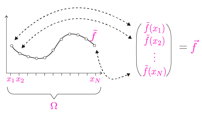^{Figure 1: a discrete function can be represented by a vector and vice versa.}

Recall that our goal is to model distributions over functions. We can model (vec{f}) using a multivariate normal distribution i.e. (vec{f} sim N(vec{mu}, Sigma)). This in turn defines a distribution over the discrete functions (tilde{f}). For example, we can draw a random function, by drawing a sample (vec{f}) from this normal distribution, and use it to define the corresponding discrete function (tilde{f}).

Representing discrete vector-valued functions using a multivariate normal distribution

In shape modelling, we are interested in modelling vector fields and not scalar-valued functions. Fortunately, this is not much more complicated. Let

$$tilde{u} : tilde{Omega} to mathbb{R}^2$$

be a discretely defined vector field. The difference to the previous case is that each component is now a vector, i.e. (tilde{u}(x_i) = (tilde{u}_1(x_i), tilde{u}_2(x_i))^T.) As before, we can identify the vector field (tilde{u}) with a vector

$$vec{u}:=(tilde{u}_1(x_1), tilde{u}_2(x_1), ldots, tilde{u}_1(x_N), tilde{u}_2(x_N))^T in mathbb{R}^{2N}.$$

Modelling (vec{u}) using a multivariate normal distribution results, as before, in a distribution over the (discrete) vector field (tilde{u}).

From vectors to function

Gaussian Processes make it possible to model a distribution over functions without choosing a discretisation up front. The intuition is the following: to model a 2D vector field, we define a Gaussian Process (GP(mu,k)) with mean function (mu : Omega to mathbb{R}^{2}) and covariance function (k : Omega times Omega to mathbb{R}^{2 times 2}). These functions define the mean deformation (mu(x)) for all the points (x in Omega) and the covariance (k(x,x’)) between the deformations for any pair of points (x) and (x’). This allows us to define normal models for functions that are defined using an arbitrarily fine discretisation. Since, in practical applications (i.e. for computer implementations), we always work with a discretisation, this is already an almost perfect situation. It allows us to choose for any application the discretisation that yields the desired accuracy.

From a mathematical point of view even more can be done. A Gaussian Process model still defines a valid distribution over functions even if we consider all the points of the continuous domain (Omega). The mathematical details are quite technical, which makes Gaussian Processes appear complicated. But the intuition that we build up for the finite domains is exactly right and we do not have to take these mathematical subtleties into account in this course.