What is Principal Component Analysis (PCA)?

A very popular method in shape modelling is Principal Component Analysis (PCA). PCA is closely related to the Karhunen-Loève (KL) expansion. It can be seen as the special case where the Gaussian Process is only defined on a discrete domain (i.e. it models discrete functions) and the covariance function is the sample covariance estimated from a set of example data. In this article, we will explain the connection between the PCA and the KL expansion in more detail, and discuss how PCA can be used to visualise and explore the shape variations in a systematic way. This can give us interesting insights about a shape family.

The Karhunen-Loève Expansion in the Discrete Case

We have seen that the KL expansion allows us to write a Gaussian Process model (u sim GP(mu, k)) as

$$u = mu + sum_{i=1}^infty sqrt{lambda_i} varphi_i alpha_i, , alpha_i sim N(0, 1).$$

Here, (varphi_i, lambda_i, i=1, ldots, infty) are the eigenfunctions/eigenvalue pairs of an operator that is associated with the covariance function (k). To fully understand this, advanced concepts from functional analysis are needed. However, if we restrict our setting to discrete deformation fields, we can understand this expansion using basic linear algebra only. Recall from Step 2.2 that if we consider deformation fields that are defined on a discrete, finite domain, we can represent each discretised function (tilde{u}) as a vector (vec{u}=(u_1, ldots, u_n)^T) and define a distribution over (tilde{u}) as

$$vec{u} sim N(vec{mu}, K).$$

(K) is a symmetric, positive semi-definite matrix and hence admits an eigendecomposition:

$$K= Phi DPhi^T = left( begin{array}{ccc} vdots & & vdots vec{varphi}_1 & ldots & vec{varphi}_n vdots & & vdots end{array} right) left( begin{array}{ccc}d_1 & 0 & 0 0 & ddots & 0 0 & 0 & d_n end{array} right) left( begin{array}{ccc} vdots & & vdots vec{varphi}_1 & ldots & vec{varphi}_n vdots & & vdots end{array} right)^T$$

Here, (vec{varphi}_i) refers to the (i)-th column of (Phi) and represents the (i)-th eigenvector of (K). The value (d_i) is the corresponding eigenvalue. This decomposition can, for example, be computed using a Singular Value Decomposition (SVD).

We can write the expansion in terms of the eigenpairs (d_i, vec{varphi}_i):

$$vec{u} = vec{mu} + sum_{i=1}^n sqrt{d_i} vec{varphi}_i alpha_i, , alpha_i sim N(0, 1).$$

It is easy to check that the expected value of (vec{u}) is (E[vec{u}] = vec{mu}) and its covariance matrix (E[(vec{u}-E[vec{u}])(vec{u}-E[vec{u}])^T] = K). Hence, we have that (vec{u} sim N(vec{mu}, K)) as required. Interpreting the eigenvectors (vec{varphi}_i) again as a discrete deformation field, we see that this corresponds exactly to a KL expansion.

The Principal Component Analysis

PCA is a fundamental tool in shape modelling. It is essentially the KL expansion for a discrete representation of the data, with the additional assumption that the covariance matrix is estimated from example datasets. More precisely, assume that we are given a set of discrete deformation fields (tilde{u}_1, ldots, tilde{u}_m), which we also represent as vectors (vec{u}_1, ldots, vec{u}_m), (vec{u_i} in mathbb{R}^n). Note that, as the vector (vec{u_i}) represents a full deformation field, (n) is usually quite large. As mentioned before, PCA assumes that the covariance function is estimated from these examples:

$$Sigma = frac{1}{m} sum_{i=1}^m (vec{u}_i – overline{u})(vec{u}_i – overline{u})^T =: frac{1}{m}XX^T,$$

where we defined the data matrix X as (X = (vec{u}_1 -overline{u}, ldots, vec{u}_m – overline{u}) in mathbb{R}^{n times m}), and (overline{u}) is the sample mean (overline{u}=frac{1}{m}sum_{i=1}^m vec{u}_i).

We note that in this case, the rank of (Sigma) is at most (m), which is the number of examples. This has two consequences: first, it allows us to compute the decomposition efficiently, by performing an SVD of the much smaller data matrix (X). Second, (Sigma) has in this case only (m) non-zero eigenvalues. The expansion reduces to (vec{u} = overline{u} + sum_{i=1}^m sqrt{lambda_i} vec{varphi}_i alpha_i, , alpha_i in N(0,1)), which implies that any deformation (vec{u}) can by specified completely by a coefficient vector (vec{alpha} in mathbb{R}^m).

Using PCA to Visualise Shape Variation

In PCA, the eigenvectors (vec{varphi}_i) of the covariance matrix (Sigma) are usually referred to as principal components or eigenmodes. The first principal component is often called the main mode of variation, because it represents the direction of highest variance in the data. Accordingly, the second principal component represents the direction that maximizes the variance in the data under the constraint that it is orthogonal to the first principal component, and so on. This property allows us to systematically explore the shape variations of a model.

We can visualise the variation represented by the (j)-th principal component by setting the coefficient (hat{alpha}_j = v) and (hat{alpha}_{i neq j} = 0) and by drawing the corresponding sample defined by

$$hat{u} = overline{u} + sum_{i=1}^m sqrt{d}_i vec{varphi}_i hat{alpha}_i = overline{u} + v sqrt{d}_j vec{varphi}_j $$

Typically, (v) is chosen such that (v in {-3, 3}), which corresponds to a deformation that is 3 standard deviations away from the mean. Figure 1 shows the shape variation associated to the first principal component for our hand example. 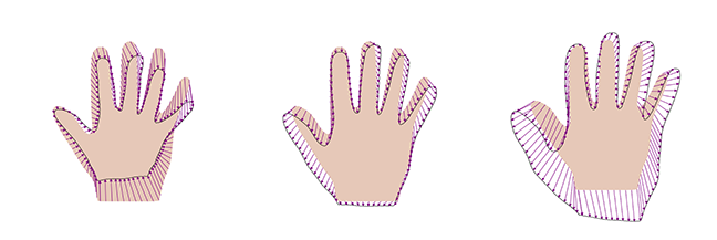^{Figure 1: the shape variation represented by the first principal component of the hand model, where the hand on the left shows a deformation with (hat{alpha}_1=-3), the middle hand shows the mean deformation ((hat{alpha}_1=0)) and the hand on the right the deformation with (hat{alpha}_1=3).}

In Scalismo Lab, visualising these variations is even simpler. The sliders that you can see in Figure 2 correspond to the coefficients in the above expansion and can be used to interactively explore the principal shape variations. 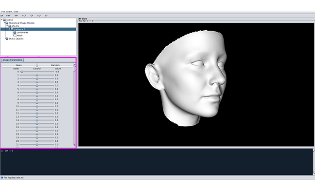^{Figure 2: visualizing shape variations in Scalismo Lab}