The importance of profit maximisation

We now need to investigate the role of profit as an incentive to allocate resources. As you’ve probably noticed, supply and demand movements are all motivated by the attraction of profit.

In microeconomics, profits are viewed as cost. This sounds counterintuitive but this is because ‘profit’ means something slightly different to accountants and economists. Think of it this way: a firm must make a profit in order to stay in business and remain competitive. Therefore, the money it brings in must be equal all its explicit costs (materials, labour and so on) plus the money needed to remain competitive (known as ‘normal profit’). Economists therefore include normal profit in total cost. This is different from the approach taken by accountants, who are interested in how much profit is being made.

So, because economists assume profits are part of total costs, they insist that total revenue (money in) must equal total costs. When total revenues are greater than total costs, you have what economists call supernormal profits.

Normal profit is when total revenue = total costs

Supernormal profit is when total revenue > total costs

The desire to make supernormal profits acts as the driver that determines the level of competition in a market, as both supplier and seller will want to make supernormal profits.

Short-term or long-term?

Earlier this week, we explored the effect of supply and demand caused by short-term changes. Short-term is defined as when one of the factors of production are fixed; this is known as the ‘short-run’ view of supply and demand. Over a longer period of time, all of the factors of production are variable, and price and demand and supply curves move backwards and forwards to reach a point of equilibrium. This is known as a ‘long-run’ view; in the long-run, all factors of production change.

For example, CV1Logistics buys labour in the form of drivers, capital as vehicles and land for the warehouse and offices. If the drivers and the vehicles are only hired for two months, but the lease on the warehouse is for five years, then this is the short-run view of the business. Drivers and vehicles can change. In the long-run, the lease will be renewed at a different price after five years.

Economics makes the assumption that, due to competition, firms will always want to maximise profits and efficiently utilise the factors of production. In the short-run, this means that profit maximisation is found where demand and supply cross at the point of equilibrium, as per the graph below. In the following graphs, cost equates to supply and revenue is demand.

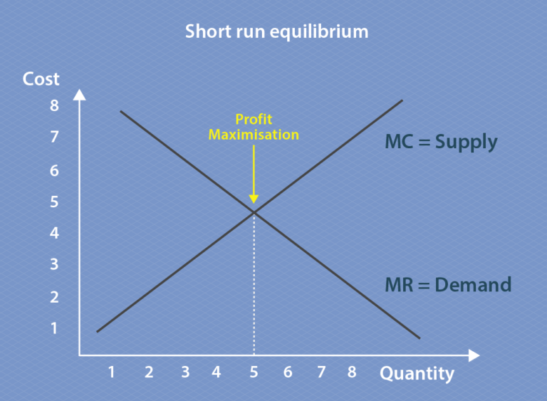
_{Adapted from Economic Help (n.d.)}

Remember, marginal cost is the cost of producing one additional unit of something, and marginal revenue is the revenue that each additional unit will generate. This means that firms will continue to increase their output as long as marginal revenue is greater than marginal cost – in other words, if the cost to produce one extra unit is less than the revenue for one extra unit. If the marginal revenue is greater than the marginal cost, then the firm will want to continue to produce because it will make a profit.

Long-run

To graph long-run demand and supply, you need to know average total costs (ATC), average revenue (AR), and marginal cost (MC) and marginal revenue (MR). MC and ATC represent supply and are always U-shaped because of diminished marginal utility. AR and MR represent demand. On the graph below, the profit-maximising output (labelled Q) is found where the MC curve crosses the MR curve, because at this point MR equals MC.

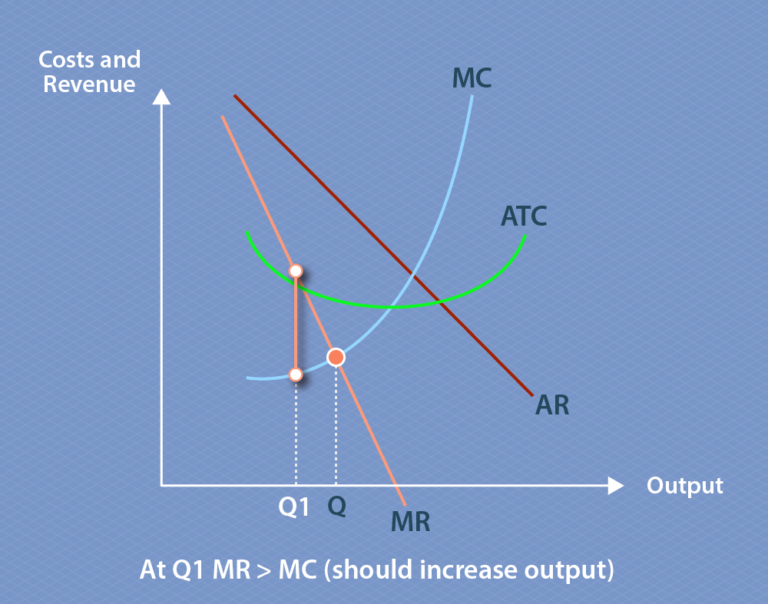
_{Key to abbreviations:
ATC – Average total cost
AR – Average revenue
MC – Marginal cost
MR – Marginal revenue}

If marginal revenue is greater than marginal cost (as at Q1 in the graph above), the firm should increase its output in order to maximise profit. For CV1Logistics, this means that when revenue is greater than costs at the marginal level, there is an incentive to provide an extra unit of product for the profit.

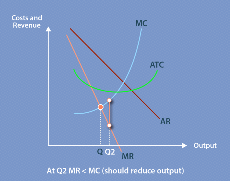
_{Key to abbreviations:
ATC – Average total cost
AR – Average revenue
MC – Marginal cost
MR – Marginal revenue}

If marginal revenue is less than marginal cost (as at Q2 in the graph above), the firm should reduce its output.

This scenario above assumes that, in the long-run, markets will regain equilibrium where MR=MC. It’s also assumed that there are multiple suppliers and sellers with easy exit and entry to the market, each with perfect knowledge. The problem with transport and logistics markets is that conditions are not perfect, because of their structure, the numbers of buyers and sellers, the effect of time and place, barriers to entry and a lack of information.

In summary

This step explains why, in the short-run, a firm would be tempted to chase supernormal profits, because marginal revenue is greater than marginal cost. In the long-run, everything goes back to normal, by returning to equilibrium and normal profit.

How this happens is dependent on the structure of the market, which we’re going to look at next. In the next section, we’ll define an ideal market and examine how markets behave when one of the conditions of an ideal market (such as perfect knowledge) is changed, which is what happens in the real world.