
Conditional Calculations

Excel has functions that allow for conditional calculations. These are calculations with conditions or criteria attached.
These functions include SUMIF and AVERAGEIFS. Functions with IF and IFS attached are widely used.
The IF functions allow you to carry out the basic function, with ONE criterion attached. Whereas the IFS functions will allow you to carry out the operation with multiple conditions attached.
The table below shows the IF and IFS functions.
How can I AVERAGE with the Conditions attached?
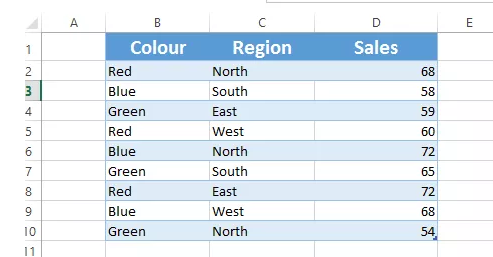
Taking the example in the image below.
Suppose you wanted to AVERAGE the sales for blue items. Using the formula =AVERAGE(D2:D14) will result in an average for all sales.
Therefore, we would need to use the function AVERAGEIF.
AVERAGEIF allows you to get the AVERAGE from one column based on criteria selected in another column. In our example, we want to AVERAGE column D and our criteria is in column B.
The syntax for AVERAGEIF is AVERAGEIF=(Range, Criteria, Criteria Range).
To solve this problem, we would use the formula:
=AVERAGEIF(B2:B10,”Blue”,D2:D10)
Where Range is the range you want to AVERAGE. In this case, column D.
The criteria is “Blue” (note how this is in “” as it is text).
The criteria range is the range where you will find the criteria. In this case, column B.
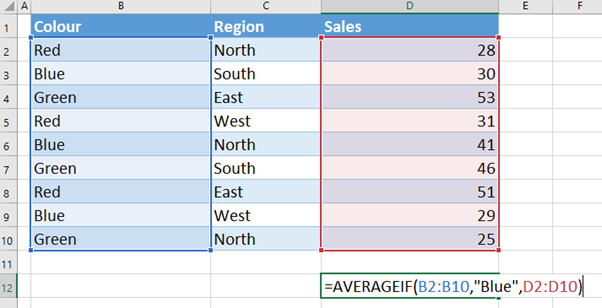
This formula will return 33.33. It will AVERAGE the sales where the color is blue.
AVERAGEIFS will allow you to average a range of data where multiple criteria are satisfied.
The syntax for AVERAGEIFS is.
AVERAGEIFS= (AVERAGE Range, Criteria Range 1, Criteria 1, [Criteria range 2, Criteria 2]….).
The average range is the first range to select in this formula. This is the range of cells that you want to average.
Criteria Range 1 is the cells containing the first criteria. Criteria 1 allows you to specify the criteria. Second and subsequent criteria can then be added.
Suppose we wanted to Average the sales where the Colour matches that of the content in cell B12. And the Region matches that of cell C12.
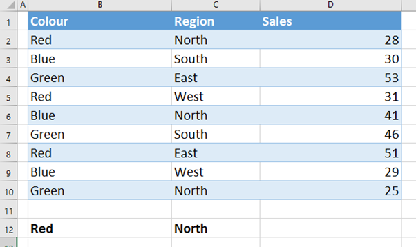
Located in range B2:B10 is the first criteria.
Cell B12 specifies the first criteria.
Located in range C2:C10 is the second criteria. Cell C12 specifies the second criteria
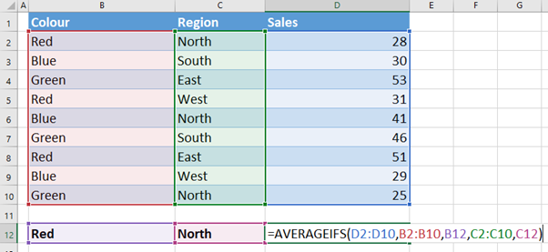
The created formula is =AVERAGEIFS(D2:D10,B2:B10,B12,C2:C10,C12)


Reach your personal and professional goals
Unlock access to hundreds of expert online courses and degrees from top universities and educators to gain accredited qualifications and professional CV-building certificates.
Join over 18 million learners to launch, switch or build upon your career, all at your own pace, across a wide range of topic areas.


