Exercise: Getting started with CATE

Now that you have learnt what CATE is, reviewed the installation of the Jupyter notebook and called CATE functionalities from it, you will move on to learn how to access, download, and perform simple visualisation and analysis operations on CCI data records of essential climate variables using CATE SaaS.

CATE provides a platform from which you can access the full archive of the Open Data Portal and carry out visualisation and analysis operations. So let us start with data sources and access.

Data Sources

After you have logged in to CATE, The DATA SOURCES panel is located at the at the top right (Figure 1).

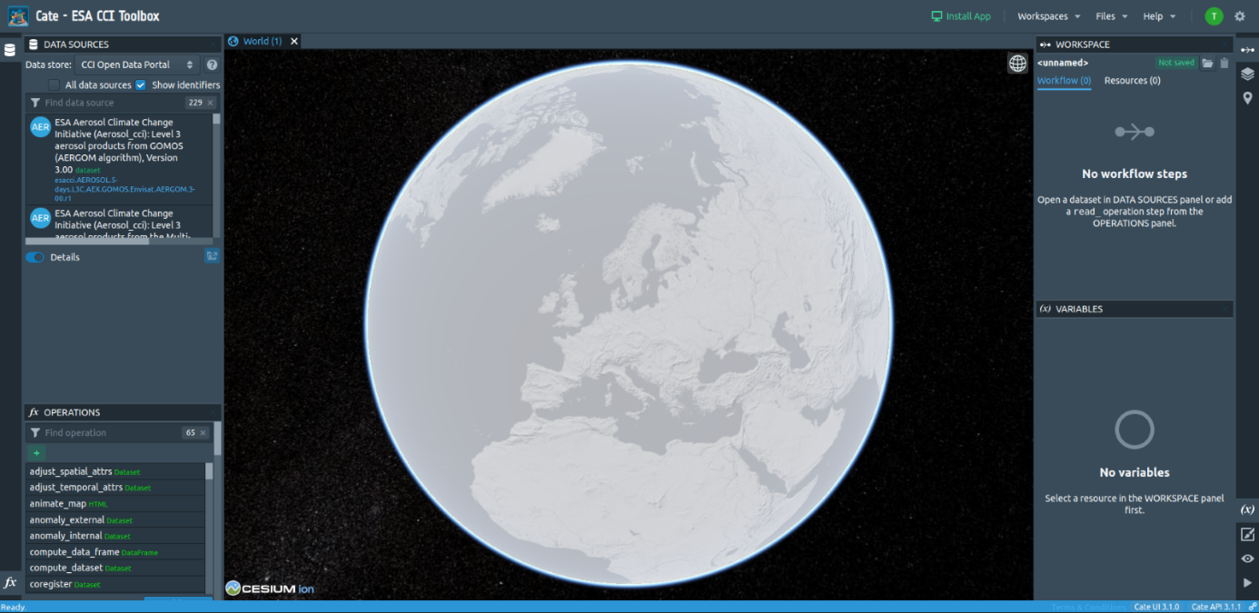
Figure 1: Open data source.

It is used to browse for and open CCI datasets. Using the drop-down list located at the top of the panel it is possible to switch between three data stores:

1. CCI Open Data Portal A remote data store that provides access to all published CCI datasets. Internally the OPeNDAP service of the ESA CCI Open Data Portal is used. Some of these datasets cannot be opened with CATE, and they are only visible when the option All data sources is checked (see the warning tooltip for more information).
2. CCI Zarr Store (experimental) A data store which provides access to ODP data that has been converted to the ZARR format. Datasets from this data store can be opened, displayed and processed significantly quicker than datasets from the CCI ODP Store, but there is only a limited number of datasets available.
3. File Data Sources A data store that allows you to store data online in your dedicated workspace. You may either upload your own data and register it as a new data source, or cache data from the CCI Open Data Portal.

Selecting a data source entry will allow displaying its details, namely the available (geo-physical) variables and the meta-data associated with the data source. Now we will explain how to work with the data sources.

Select from the ESA CCI Open Data Portal the dataset with the title ESA Aerosol Climate Change Initiative (Aerosol_cci): Level 3 aerosol products from the Multi-Sensor UV Absorbing Aerosol Index (MS UVAI) algorithm, Version 1.7. CATE will load data explaining the data source in the Details section of the panel (see Figure 2). There you can also find a link to the dataset’s catalogue entry.

The full archive of data is located at https://climate.esa.int/odp/. There you might also find datasets that are not yet accessible via the ODP/Cate.

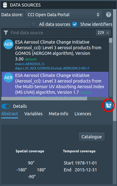
Figure 2: The Data Source Panel

Next, open the data by clicking on the Open Data Source button (indicated by a red circle in Figure 2). You can select (and you are advised to do so) region, time, and variable constraint (Figure 3). Select a small region and the full-time record of observation. You also have the option to cache the data and assign a new name to it. If you cache it, a copy of the data source will be put into the File Data Sources data store.

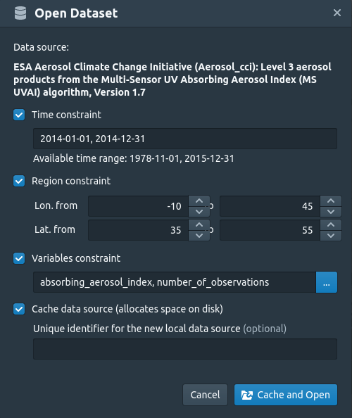
Figure 3: CATE’s Open Dialog

If you have selected a spatial, temporal or variable subset, a subset will be cached. If you close Cate and log in back at some alter point, the cached data source will still be available. Working on cached data is faster, but the caching process itself takes some time, depending on the amount of data to be cached.

After confirming the dialog, a download task will be started. Once the download is finished, a notification will be shown, and the dataset will be displayed on the world view (Figure 4). If you had checked the caching option, a new local data source will be available in the File Data Sources data store.

Figure 4: The Aerosol Dataset after opening

Data Analysis

This section shows how you can access CCI data and use CATE operations to visualise and analyse the data. By doing so, the Absorbing Aerosol Index will be explained.

Open and visualise data

By now you should have opened the Aerosol dataset. Note that you can open it multiple times, with, e.g., different subset parameters. The following steps are performed best with a subset of a temporal period of about one year.

At the top of the right panel you see the workspace with an overview about the operations you performed and its results. Right now, it should list the times you opened a dataset.

At the bottom of the right panel is a list of variables contained in this data source. You can select any variable. In the panel, detailed information about the variable is shown. If the variable has latitude and longitude dimensions, it will be directly visualised on the globe. You can explore any region on earth by rotating the globe and zooming into areas of interest.

Choose any point on earth and right-click to place a point marker (Figure 5). A green rectangle will indicate that this placemark is now selected.

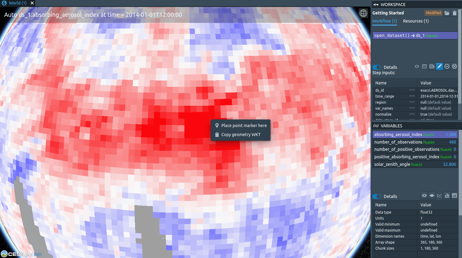
Figure 5: Visualising with CATE and placing a point marker.

In the VARIABLES panel on the right, click Create a time-series plot from selected placemark (Figure 6). When computation has finished, a plot will be opened (Figure 7).

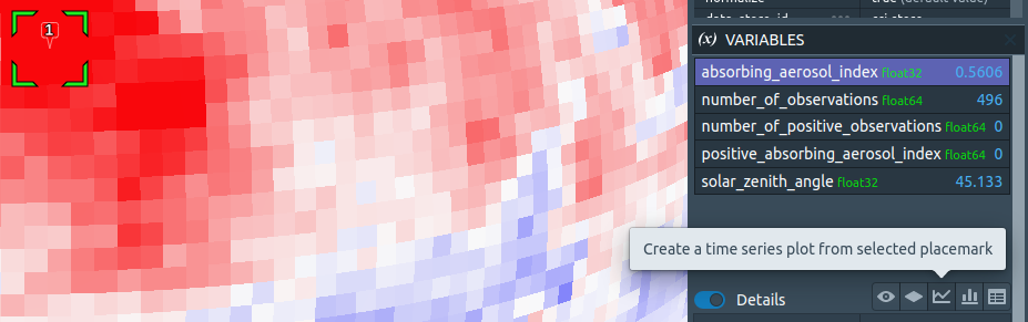
Figure 6: Create a time series plot from the selected placemark.

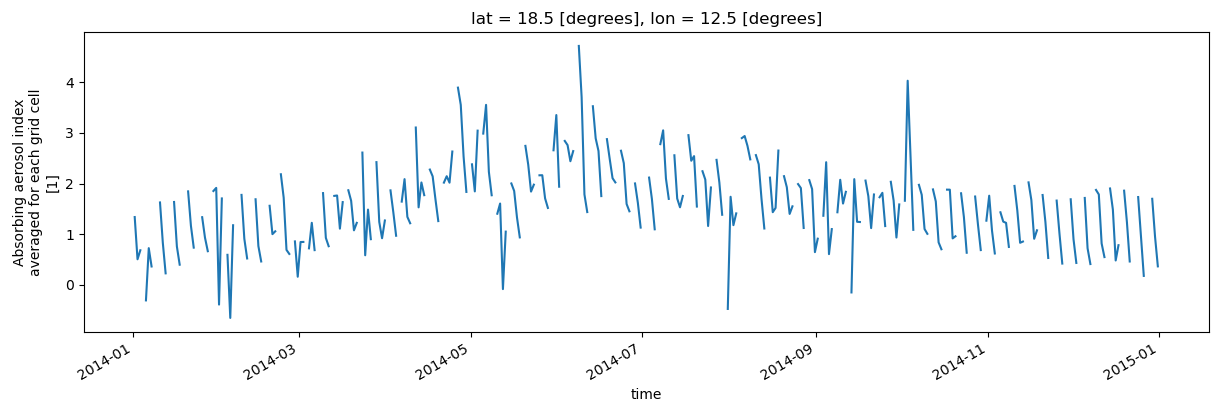
Figure 7: The Time-Series for the selected place marker

You can compare with a different region of the world by putting another placemark (Figure 8) and creating a time series for it. A new tab with the time series plot of the second place marker will appear (Figure 9).

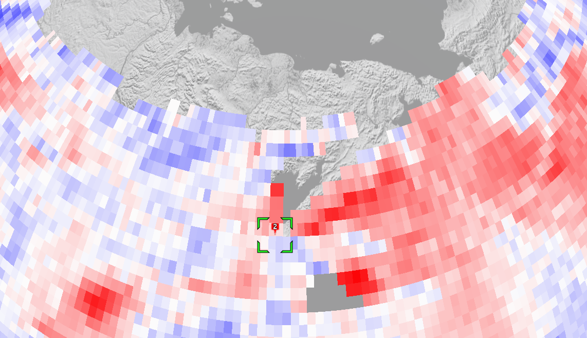
Figure 8: Placing a second marker

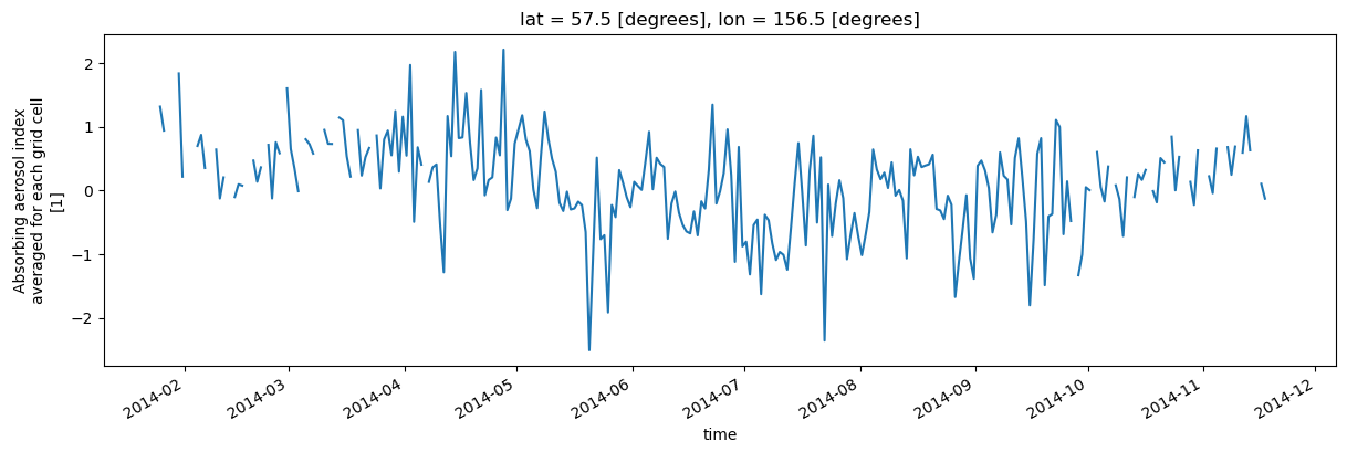
Figure 9: Time series at the second place marker

There are two main features to learn from this example:

1. The Absorbing Aerosol Index (AAI) is a qualitative quantity that shows the presence of absorbing aerosols. In this case, the ultraviolet (UV) spectral range is used to detect the presence of UV-absorbing aerosols in the atmosphere. Positive values indicate the presence of absorbing aerosol like smoke and dust while small or negative values represent non-absorbing aerosols and clouds. The values of AAI are dependent on aerosol properties but also on sensor characteristics, and retrieval conditions (solar zenith angle and surface albedo).
2. Different locations will have different values and time series. For example, comparing the time series in Figures 6 and 7, we can observe that in Europe (place marker 1), scattering aerosol is present.

To appreciate the presented time series, you can plot the histogram of the global climatology values of AAI (Figure 9).

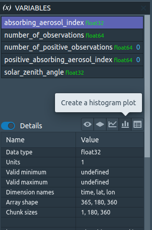
Figure 10: Create a histogram plot

Now one can immediately notice that in our example the time series of Figure 7 and Figure 9 represent extreme values. The values of Figure 7 are located at the right-end of the histogram, whereas the values of Figure 9 are located at the left-end.

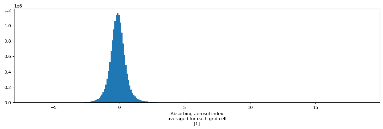
Figure 11: Histogram of the global climatology values of absorbing aerosol index.

Up next

Congratulations, you have reached the end of this activity and the week! Now let us review the knowledge you acquired during this first week.