Introduction to climate data

Climate data can take many different forms. Here are some of the main sources along with their advantages and limitations.

Site-based meteorological instruments

Conceptually, the most straight-forward source of climate data is derived from in-situ measurements using dedicated meteorological instruments (a record of temperature or precipitation observations at a particular location). Provided the observing instrument is well sited, well maintained and well calibrated, such measurements offer a high quality record of the local weather conditions for the site. Many have the added advantage of having been in place for decades so that historical data is available. Networks of quality-controlled standardised observations of this type are typically maintained by National Meteorological and Hydrometeorological Services and form part of the World Meteorological Organisation’s ‘Global Observing System’ which is used in operational weather forecasting around the world.

The limitations of such observational networks relate to the physical locations of the recording sites. They may be sparsely located, may not record the measurement you need, and the nearest observing station to the site you’re interested in may be in a poor position.

For example, a wind farm developer wishes to estimate wind speeds over part of a hill – the yellow area in the diagram below.

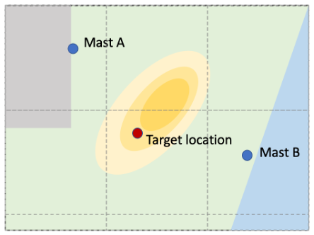
Two nearby observation stations (Masts A and B) are available but both lie on the surrounding plains (green area) rather than the hill itself. Neither mast is therefore likely to provide a good estimate of wind speed over the hill and wind speed behaviours at both sites may be influenced by confounding factors. The recordings for Mast A will be influenced by the nearby city (grey area), and in the case of Mast B, coastal affects due to the nearby ocean (blue area).

Even at the best maintained sites the surrounding conditions may change (for example, tree growth or new buildings) and instruments are replaced over time, both of which create the potential for spurious trends, disruptions and discontinuities in the records produced. New observation sites can, of course, be installed (to target a particular location or property of interest) but records can only be created in real-time – it’s not possible to create a long historic record of in-situ weather observations retrospectively.

Remote-sensing and proxy observations (including satellites)

An alternative source of weather and climate data is constructed from indirect observations. Over the last few decades, satellite-based meteorological observations have revolutionised weather forecasting science, offering comprehensive and high-quality records spanning large areas of the globe. And studies of tree rings and ice cores (‘proxy’ data) have begun to provide deep, long-term perspectives on climate change and variability.

Meteosat Third Generation (MTG) Imaging and Sounding satellites.© ESA.

The limitation is that they rely on calibration models which ‘translate’ the property observed – typically, electromagnetic emissions spectra received by a satellite or an isotopic ratio in an ice core sample – into an estimate of particular climate properties. In many situations these assumptions can be very hard to test so the climate data produced require careful interpretation.

Another limitation of this type of observation (like the site-based meteorological instruments) is that they are intrinsically backward-looking: they reveal only a single weather history (the weather history which actually occurred), rather than revealing either a range of different weather histories that could have occurred or how the climate might change in the future. To address these limitations a different type of data is needed, derived from climate simulations.

Numerical models and simulations

The concept of creating a numerical (ie, mathematical) model for forecasting weather has a long history, dating back to before the advent of modern computing with Lewis Fry Richardson’s 1922 ‘Forecast Factory’. These models can be used to produce comprehensive, high quality 3-dimensional gridded meteorological simulations. They are used extensively for both operational weather and climate forecasting (days to months and even years ahead) and climate change projections (usually several decades ahead). You’ll read how these models are constructed in Step 2.5.

A major advantage of numerical models is that they can, in principle, produce a complete suite of meteorological data outputs across very long simulations at very high resolution (ie, a fine-mesh grid), spanning the entire globe or targeted regions. It’s also possible to use such models to predict the future and explore the deep past by simulating how weather conditions might be affected by changing climate drivers. For example, the effect of increasing concentrations of atmospheric greenhouse gases on climate in the near future can be estimated, or the impact of orbital cycles associated with past ice ages can be explored. The models can also be used to create alternative ‘weather scenarios’ – realisations of weather which are different to recorded weather but nevertheless consistent with historical climate drivers. These scenarios are particularly useful for examining the properties of rare and extreme weather events.

Numerical models also have their limitations. They are all subject to biases and deficiencies that limit the quality of their output, which can be difficult or even impossible to fully evaluate. They are also computationally expensive and, while archives of model simulations are available (eg, the major international efforts to produce the CORDEX and CMIP archives of climate model simulations and national initiatives such as the UK Climate Projections), they may require further processing to meet the needs of a particular business.

Reanalyses

Finally, ‘reanalyses’ are comprehensive, 3-dimensional, gridded, historic, weather datasets, usually with global coverage and spanning several decades into the past. Reanalyses combine state-of-the-art numerical models with historical observations through a process known as ‘Data Assimilation’ – a concept closely related to machine learning.

This simplified schematic represents the production of a meteorological reanalysis.

Click to expand.

The general process works as follows. We have, for example, a set of meteorological observations relating to a particular ‘validity’ time, 06Z (Observations 06Z). We also have a short-range numerical weather prediction forecast relating to the same validity time (NWP 06Z) available (the forecast was launched from a set of observations taken just six hours earlier, Observations 00Z). Both the forecast and current observations are good estimates of the true meteorological state at 06Z but neither is perfect and so they differ. The ‘data assimilation’ (DA) process is used to blend these two information sources together, to produce a single overall best estimate (Atmospheric state estimate 06Z). This new estimate is then used as the starting conditions for a new short-range forecast (targeting a validity time of 12Z; NWP 12Z), and the DA process is repeated to combine the new forecast, with a new set of observations for 12Z (Obs 12Z). This process is then repeated many times, stepwise, forward in time.

There are two broad types of reanalysis. One focuses on the modern era (typically 1950-1980 onwards) and assimilates a full range of meteorological observations. The other type assimilates a reduced set of site-based observations but achieves a longer coverage from around 1900 onwards.

By construction, reanalyses can, to some extent, be considered as a ‘best estimate’ of the atmospheric circulation over the entire globe. They also provide a full suite of data on the associated local meteorological conditions (eg, precipitation, temperature, wind speeds) and are typically available on a grid box scale of tens of kilometres and an hourly timescale. They therefore have many uses in climate risk assessment.

It’s important to recognise, however, that even reanalyses have limitations. Their limited resolution (grid box size) can be problematic for assessing highly localised meteorological conditions (like the wind speeds over the hill that the wind farm developer needed at the beginning of this article. In the figure, the dotted lines are indicative of a typical reanalysis grid-box size and would clearly fail to adequately capture the complex terrain involved). Changes in observational systems can also introduce spurious trends in the estimated variables (like the atmospheric state estimates above). Deficiencies in the numerical weather prediction model can also introduce biases and errors when simulating surface properties such as precipitation.

Summary

There are many sources of climate data which can be used to estimate and manage climate risk. However, no single data source is perfect as they all have their advantages and limitations. It’s vital, as part of your planning process, to assess and consider which best meets your needs and if it’s ‘fit for purpose’.

In the next Step, you’ll reflect on what data sources might fit your particular business purpose.

Optional further reading

Charlton-Perez, A. and Dacre, H. (2011) Lewis Fry Richardson’s forecast factory – for real. Weather, 66 (2). pp. 52-54.

Lynch P. 2006. The Emergence of Numerical Weather Prediction. Cambridge University Press: Cambridge, MA.

Richardson LF. 1922. Weather Prediction by Numerical Process. Cambridge University Press: Cambrdige, MA. Reprinted 2006 by Cambridge University Press with a new introduction by Peter Lynch.