Our first model

In the last step we found a promising pattern in the dimensions of the paintings which seem to fall into two broad clusters. We would like to use this knowledge to build a model that will enable us to infer a decision procedure that tells us for every width and height data point (w, h) whether it is a landscape painting, a portrait painting or something else. To that end, let us define the ratio of a painting as the fraction.

[r=frac{height~of~painting}{width~of~painting}]

A painting whose height is equal to its width has a ratio of one, a painting whose height is greater than its width will have a ratio greater than one ( ≥1 ) and a painting that is wider than tall will have a ratio less than one ( ≤1 ).

We expect the width of a landscape painting to be larger than its height, hence, in this case, (r) should be smaller than one (the numerator is smaller than the denominator). The opposite is true for portrait paintings, we therefore would expect (r) to be larger than one. As so often in life, reality is messy and we can easily find counterexamples in the dataset:

Sir John Everett Millais, Bt, “Dew-Drenched Furze” (1889) has a ratio of ≈ 1.41 and Sir Brooke Boothby, “Joseph Wright of Derby” (1781) has a ratio of ≈ 0.72. Photo © Tate.

As the famous 20th century British statistician, George Box (1976), said: ‘All models are wrong, but some are useful’. A model provides us with an explanation of what we see in our data, so for the explanation to be understandable, the model needs to be simple. This brings us to the fundamental tension in designing models: a simple model will get many things wrong, but also be easy to interpret. A complicated model will be closer to the data, but it will be hard to understand.

Let us formulate the model we have outlined above. We choose two parameters (t_{port}) ≥1 and (t_{land}) ≤1, and label a painting according to its ratio (r) as follows:

• If (r) ≤ (t_{land}) then we label the painting as “landscape” (L),

• If (r) ≥ (t_{port}) then we label the painting as “portrait” (P),

• And else we label our painting as “other” (O).

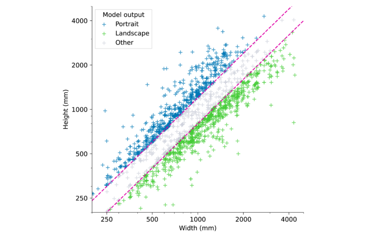
We choose these two threshold parameters to reflect the uncertainty in our decision, so that for a ratio very close to one we cannot be certain whether the painting is a landscape or a portrait. We can optimise the two thresholds later, for now let us simply choose (t_{land})=0.8 and (t_{port})=1.2 as our first order approximations. We can visualise these decision boundaries, which separate the three classes L, P and O, in a scatter plot (note that we again use a log-log plot to enhance the readability of the plot):

Click image to expand.

Our very simple model now classifies the data points into three classes (L,P, and O). The two decision boundaries correspond to the lines (b_{port}(w) = t_{port}w) (top line) and (b_{land}(w) = t_{land}w) (bottom line). Points above (b_{port}(w)) are classified as P, points between (b_{port}(w)) and (b_{land}(w)) as O, and points below (b_{land}(w)) as L, where ‘w’ is the width of the painting.

Your task

First model (15 mins)

Now that you have been introduced to the basic model, your task is to interact with the ‘ratio model’ by choosing the decision thresholds. You will choose the upper and lower decision boundary and output a plot and the corresponding confusion matrix.

What are the best thresholds in your opinion? Let everyone know in the comments section.

Visit the Jupyter Notebook.

References

_{Box, G. E. P. (1976). Science and statistics. Journal of the American Statistical Association, 71(356), 791–799. DOI:10.1080/01621459.1976.10480949.}

_{TATE. (n.d.). Sir John Everett Millais, Bt. Dew-drenched furze, 1889–90. Web link}

_{TATE. (n.d.). Joseph Wright of Derby, Sir Brooke Boothby, 1781. Web link}