Scatter plots in Matplotlib

Scatter plots are drawn with the Axes.scatter method. Similar to the plot method, they take at least two arguments, the x- and y-positions of the data points, as lists, arrays, or DataFrames.

In this course, we will be using various data sets and one of them is the Iris data set, which will be of the petal length versus the petal width to demonstrate the scatter plot. Download the zip file at once and save the individual CSV files with the same name under the same folder where your notebook lives. Let us use the iris.csv for this activity.

Download: Iris.csv

Alternatively, you can also access the file from the Github source. [1]

Step 1

This time you will import Pandas library for working on our scatter plot and the Iris.csv file along with setting the figures and axes for the chart.

Code:

import pandas as pd

iris_data = pd.read_csv(”iris.csv”)
versicolor = iris_data[iris_data.variety == “Versicolor”]
setosa = iris_data[iris_data.variety == “Setosa”]
virginica = iris_data[iris_data.variety == “Virginica”]

fig, ax = plt.subplots()
fig.set_size_inches(8, 8)

Step 2

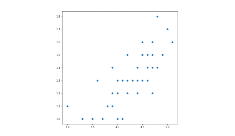
Next, you will just draw the Versicolor data.

Code:

points = ax.scatter(versicolor[”petal.length”], versicolor[”petal.width”], label=”Versicolor”)

Output:

Click to enlarge

Step 3

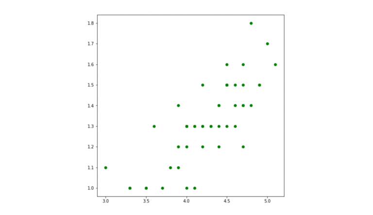
The return value is a collection of the points that were plotted, and we can then use that reference to make changes to the way points are displayed. For example, we can change the colour of the plots.

Code:

points.set_facecolor(”green”)

Output:

Click to enlarge

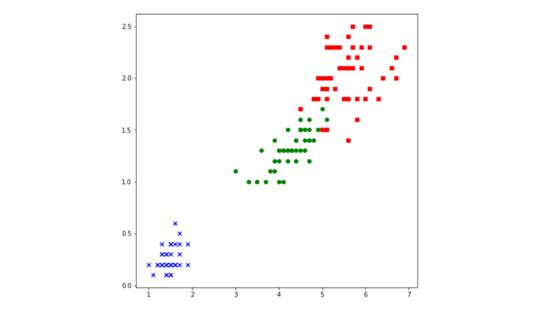
Isn’t that amazing? Similarly, you can even set attributes when the points are drawn. For example, try setting the colours and marker style on the other points.

Code:

ax.scatter(setosa[”petal.length”], setosa[”petal.width”], label=”Setosa”, marker=”x”, facecolor=”blue”)
ax.scatter(virginica[”petal.length”], virginica[”petal.width”], label=”Virginica”, marker=”s”, facecolor=”red”)

A marker style of x sets the marker to a cross, while s means square.

Output:

Click to enlarge

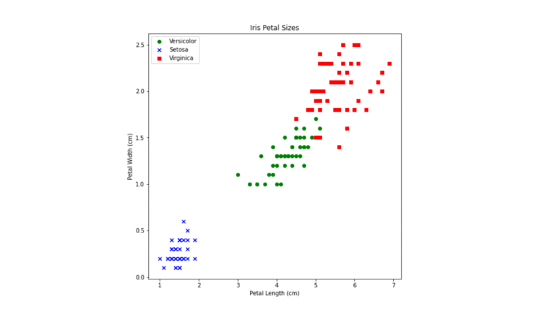
As with other types of plots, we can set the title and axis labels, then add a legend (using the same methods we’ve already seen).

Code:

ax.set_xlabel(”Petal Length (cm)”)
ax.set_ylabel(”Petal Width (cm)”)
ax.set_title(”Iris Petal Sizes”)
ax.legend()

Output:

Click to enlarge

You could also continue customising the plot by adjusting the axes scales and tick marks using the same functions we’ve seen for other plot types. The complete documentation for the scatter method can be found in the link. Read through this documentation to improve your understanding of scatter plots.

Refer to: Scatter plot documentation [2]

After creating all these wonderful plots, how do I save them?

You will learn that along with automating the plot generation with Python scripts in the subsequent step.

References

1. Github dataset [Internet]. Github; [date unknown]. Available from: https://github.com/mwaskom/seaborn-data

2. matplotlib.axes.Axes.scatter [Document]. Matplotlib; [date unknown]. Available from: https://matplotlib.org/3.1.1/api/_as_gen/matplotlib.axes.Axes.scatter.html