
Analysing segregation data
In this step, and the exercise step which follows, we are going to focus on analysing segregation data in more detail.
These steps will be helpful for learners who may have to evaluate segregation data in their own clinical practice. If this is not relevant for you, feel free to move ahead to ‘Part 7: Other databases and Other data (phenotype)’.
The ACMG guidelines1 state that cosegregation of a variant with disease can be used as evidence in support of pathogenicity (PP1). Similarly, nonsegregation of a variant with disease can be used in support of a benign classification (BS4).

The guidelines also suggest that increasing amounts of segregation data can be used to up-grade the strength of PP1 from supporting evidence to moderate or strong evidence.
So, what constitutes enough cosegregation data for use in support of pathogenicity of a variant, or even to justify an upgrade to moderate or strong?
In 2016, Jarvik and Browning produced a paper2 to address this issue, with a set of easily implemented quantitative guidelines to analyse cosegregation of a variant with a disease, to be used in variant analysis by clinicians and clinical scientists.
In this step we will consider the main points from the guidelines,2 and work through some examples of how they can be used to analyse segregation data from a pedigree. In the following exercise step you will then have a chance to try it for yourself.
Analysing segregation data – key points:
The model requires the following assumptions to be met:
- Full penetrance of the condition, with no phenocopies.
- The allele is sufficiently rare that all occurrences of the variant in the pedigree are inherited from a common ancestor, rather than entering the pedigree multiple times from more than one source.
Segregation data can be analysed from just one family with multiple affected members, or from individuals across multiple affected families who carry the same variant and with the same condition.
A simple probability is calculated that the observed variant-affected status data in the pedigree(s) occurred by chance.
The lower this calculated probability, the more likely it is that the variant is co-segregating with the condition in the affected members, rather than the observed distribution being simply due to chance.
Cut-offs are given for this calculated probability, to define what constitutes supporting, moderate or strong evidence for pathogenicity.
| Evidence level | Data from single family | Data from multiple families |
|---|---|---|
| PP1_Supporting | ≤1/8 (≤0.125) | ≤1/4 (≤0.25) |
| PP1_Moderate | ≤1/16 (≤0.06) | ≤1/8 (≤0.125) |
| PP1_Strong | ≤1/32 (≤0.03) | ≤1/16 (≤0.25) |
Table 1: Thresholds for the probability of the variant-affected status data occurring by chance that can be used at each evidence level in support of pathogenicity (Supporting, Moderate or Strong) for data from a single family or multiple families.
Note that the cut-offs are more stringent if the data come from a single family, rather than multiple families, due to concern that in a single family there is greater chance that the evidence could be due to physical linkage (linkage disequilibrium) between the observed variant and an unknown causative variant.
So how do we calculate the probability that the observed variant/affected status data occurred by chance?
This is best explained by example…
Consider a scenario where you have a proband and parent, both affected by the same dominant disorder, and both carrying the variant of interest, but no other genomic data available from the family (Pedigree 1).

Click to expand
Pedigree 1. Affected individuals are filled, unaffected are unfilled. A plus sign indicates that the individual carries the variant of interest. The proband is identified with an arrow.
Given that the proband carries the variant (we therefore consider their probability as ‘1’), the probability that their affected parent also carries the same variant purely by chance, rather than due to the variant being causative of the condition, is ½. (This reflects the 50:50 chance of the parent passing on the allele containing the variant of interest to the child, as opposed to the other allele in the autosomal pair.)
The overall probability of the observed variant/affected status data occurring by chance (rather than because the variant is causative of the condition) is therefore: 1 (proband) x ½ (affected parent) = ½
Since there is a relatively high probability of this data occurring purely by chance, this amount of segregation data would not meet the cut-off of ≤1/8 for data from a single family needed to be used as supporting evidence for pathogenicity in classification of the variant (see Table 1).
Now imagine the proband also has an affected sibling, who is also found to carry the variant of interest (Pedigree 2).

Click to expand
Pedigree 2. Affected individuals are filled, unaffected are unfilled. A plus sign indicates that the individual carries the variant of interest. The proband is identified with an arrow.
The combined probability of this occurring purely by chance is now lower: 1 (proband) x ½ (affected parent) x ½ (affected sibling) = ¼.
We can generalise this in an equation, as follows:
The probability, N = (1/2)m, where m is the number of meioses of the variant of interest that are informative for cosegregation.
In the above example, N = (½)2 = ¼.
Again, this would not be enough evidence to use PP1 at a supporting level (Table 1).
The absence of the variant of interest in an unaffected family member can also be used as cosegregation data.
Consider that this time there is also an unaffected sibling, who is tested and found not to carry the variant shared by their affected parent and siblings (Pedigree 3).
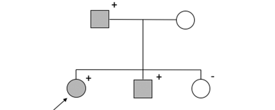
Click to expand
Pedigree 3. Affected individuals are filled, unaffected are unfilled. A plus sign indicates that the individual carries the variant of interest, a minus sign indicates that the individual does not carry the variant of interest. The proband is identified with an arrow.
The combined probability of this occurring by chance is now lower again:
1 (proband) x ½ (affected parent) x ½ (affected sibling) x ½ (unaffected sibling) = ⅛.
This can also be expressed as the product of the number of informative meiosis, i.e. N = (½)3 =⅛.
With this added data from the unaffected sibling, we have now reached the ≤1/8 threshold which enables us to use this as supporting evidence for pathogenicity (PP1) of this variant (Table 1).
Consider now a family in which there are multiple members affected by a dominant disorder, and you have genomic data for only some of the family members (Pedigree 4).
In this case, it is important to remember the underpinning assumption that a very rare variant within a family has been inherited from a common ancestor, rather than entering the pedigree from independent sources.
This allows us to assume that relatives for whom we may not have genomic data but who connect those carrying the variant of interest are also carriers.

In this case, we can use the following data in the analysis:
- There are three family members who are affected and have had genetic testing that has identified the same rare variant – the proband (III-1), their affected parent (II-2) and first cousin (III-3).
- We can also assume that the affected maternal uncle (II-3), who is deceased and for whom we have no genomic results, was a carrier, because his son (III-3) is a carrier and must have inherited the variant from him.
- The proband’s sister (III-2) does not carry the variant of interest and is unaffected.
- The proband’s maternal aunt (II-6) was apparently affected but is deceased and we have no genomic results for her. She does not have any affected children so we can’t assume that she carried the variant, so she cannot be included in our calculation. However, her unaffected daughter (III-4) has been tested and does not carry the variant.
Since one of her grandparents must have carried the variant, the probability of her being a non-carrier by chance would be 1 minus the probability of her being a carrier i.e. 1 – (½ x ½) = ¾. This probability can therefore be added to our total reckoning.
This gives us the following calculation for the probability of this observed variant/affected data occurring by chance:
1 (proband, III-1) x ½ (affected carrier parent, II-2) x ½ (affected carrier cousin, III-3) x ½ (obligate carrier uncle, II-3) x ½ (unaffected non-carrier sibling, III-2) x ¾ (unaffected non-carrier cousin, III-4) = (½)4 x ¾ = 12/256 ≅ 1/21
Since the data are from a single family, this ≅1/21 probability meets the ≤1/16 threshold for use as PP1_Moderate evidence in support of pathogenicity (see Table 1).
Combining data from multiple families
When combining segregation data from multiple affected families with the same condition and carrying the same variant of interest, the number of informative meioses from across all the families can be added together to give a value for m.
For example, if you have three separate pedigrees, all with an affected child and an affected parent sharing the same variant of interest across all the families in a dominant disorder, there is one informative meiosis for each pedigree, m=3, and N = (½)3 = ⅛.
Since the data for this variant come from multiple families, we are able to use less stringent thresholds for the evidence levels than for a single family and ⅛ meets the cut-off of ≤1/8 for use at the PP1_Moderate level (Table 1).
Recessive and X-linked conditions
So far we have only considered autosomal dominant conditions, but this method can also be employed for autosomal recessive and X-linked conditions.
In the context of an autosomal recessive condition, if two affected siblings carry the same two variants in trans, the calculation would be: 1 (proband) x ½ (probability of sibling carrying the first variant by chance) x ½ (probability of the sibling carrying the second variant by chance) = ¼.
Cosegregation of an X-linked pedigree can be similarly calculated by assigning the proband a probability of one, then calculating the probability of the observed segregation in other family members.
For example, for an affected male proband with one affected brother carrying the same variant and one unaffected non-carrier brother, N = ½ x ½ = ¼.
Use of segregation data to support a benign classification
It is important to remember that segregation data can also be used as strong evidence for a benign classification (BS4).
In the case of a fully penetrant dominant disorder, a single unaffected individual who carries the variant of interest is considered sufficient evidence for nonsegregation of the variant with the condition.
However, nonsegregation can be difficult to establish in the case of late onset conditions, or those with reduced penetrance. Care must be taken to rule out mild presentations in apparently unaffected family members, and biological family relationships must be confirmed.
Furthermore, for more common conditions, phenocopies (individuals with the same phenotype due to a different genetic or non-genetic cause) may act as a confounder (e.g. a carrier of a BRCA1 variant who has a sister who does not carry the variant but is affected by sporadic breast cancer).
So, in summary, caution should be employed before using nonsegregation data to support a benign variant classification.
In the next step you can put what you have learnt into practice by evaluating a series of pedigrees and deciding whether the data can be used to support a pathogenic variant classification and, if so, at what level.
References
1 Richards S, Aziz N, Bale S, et al, ‘Standards and guidelines for the interpretation of sequence variants: a joint consensus recommendation of the American College of Medical Genetics and Genomics and the Association for Molecular Pathology’. Genet Med. 2015;17(5):405-424. doi:10.1038/gim.2015.30
2 Jarvik GP, Browning BL. Consideration of Cosegregation in the Pathogenicity Classification of Genomic Variants. Am J Hum Genet. 2016;98(6):1077-1081. doi:10.1016/j.ajhg.2016.04.003
For those taking part in the external course evaluation please follow this link to provide feedback for the step.
Interpreting Genomic Variation: Fundamental Principles


Interpreting Genomic Variation: Fundamental Principles
Reach your personal and professional goals
Unlock access to hundreds of expert online courses and degrees from top universities and educators to gain accredited qualifications and professional CV-building certificates.
Join over 18 million learners to launch, switch or build upon your career, all at your own pace, across a wide range of topic areas.


