Grover’s algorithm consists of two parts: marking and diffusion. First, we will discuss a little more formally the structure introduced in the previous Step, then we will see some examples of mark routines in this Step, and discuss diffusion and performance in the next Step.

Overview of the Algorithm

Start with a function (f(x)) that takes some input (x) and returns TRUE or FALSE. Your goal is to find a value of (x) for which it returns true. (For the moment, assume there is only one value for (x) that returns true, although that doesn’t necessarily have to be so.) For our purposes here, assume that the characteristics of the problem are such that the number of possible values for (x) is large, and you have no way of making an informed guess what might be a good value for (x). Even if you calculate (f(x)), it only gives you true/false, no “that was close” or anything that guides you toward a better guess for (x) next time. All you can do is keep trying different values for (x).

These kinds of problems are often called randomized database search problems, though I (Van Meter) am not wild about this particular term. We can rephrase them to the question, “For what value of (x) does (f(x) = k)?” Unstructured problems like this are difficult to solve efficiently. With no ability to direct your search, on average, you would expect try half of the possibilities for (x) until one returns true.

Grover’s algorithm allows you to perform the calculation of that function fewer times. If (N) is the number of possible values for (x), you must calculate (f(x)) only (O(sqrt{N})) times, and it will give you your answer with >50% probability (usually close to 100%).

Of course, in accordance with our basic approach to quantum algorithms, this effect is achieved using interference, which depends on the phase of the states. Lov Grover’s fundamental insight is that it’s possible to implement an “inversion about the mean” operation that creates this interference, which we will see in the next Step.

To achieve this, we need two routines: a mark routine that labels our answers as good or bad, and a diffusion operator that “smears out” our probability amplitude over the other dials. The exact effect of that diffusion depends on whether or not that state was marked.

The Mark Routine

The mark routine tests whether or not we have found the answer to our question. Of course it is implemented using the unitary gates we have already described, but this is largely a task with a simple classical analog, calculating (f(x)) and returning true or false.

In our chess example, (x) might be a sequence of moves, and (f(x)) a function that returns true if the sequence results in a win and false if it results in a loss. For argument’s sake, let’s assume there are four possible moves, and exactly one of them results in checkmate (a win for us).

To find the best move classically, in the worst case we might have to try four times before hitting the win, and the average number is 2.5 times. If we use a quantum computer with two qubits and Grover’s search algorithm, we can find the answer using our check operation only one time.

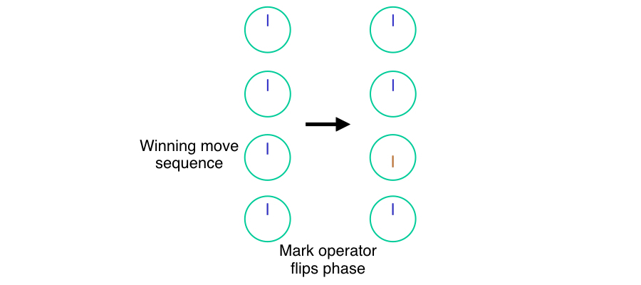
To start the algorithm, we set up a superposition of all four states. (To encode four states using qubits, of course we use two qubits, so that the numbers (00), (01), (10), and (11) each represent one of our move sequences.) In our dial notation, that means our register (|xrangle) has four dials, each with the same amplitude and phase. This initialization gives us the set of four dials on the left in the diagram at the top of this article. (Again here, we are not using exactly correct vector lengths in the dials, in order to keep them visually easy to understand.)

Second, we execute our mark routine, which flips the phase (changes the phase by (pi)) of only states where (f(x)) is true. This is the transition corresponding to the arrow in the diagram. The state corresponding to the winning move sequence, shown in orange, now points down, opposite the phase of the three losing moves.

It’s important to note here that we can construct a circuit using the gates we have already described to make our function (f) even if we do not know the answer; the function must know how to recognize an answer, but does not include that information directly. Otherwise the algorithm would just be confirming what we already know!

希望の状態をマークする

Groverのアルゴリズムは、マーキングと拡散の2つの部分で構成されています。 まず、前のステップで紹介した構造を少し厳密に議論し、次にマークルーチンの例を見て、次のステップで拡散とパフォーマンスについて議論します。

アルゴリズムの概要

まずは何らかの入力(x)をとり、真偽値(真または偽)を返す関数(f(x))について考えましょう。 あなたの目標は、(f(x))が真を返す(x)の値を見つけることです。 （現時点では、必ずしもそうである必要はありませんが、真を返す(x)の値が1つしかないと仮定します。） ここでは、問題の特性として(x)の取りうる値の数が多く、良いと思われる(x)が何であるかを情報に基づいて推測する方法がないと仮定します。 たとえあなたが(f(x))を計算したとしても、それはあなたに真偽を提供するだけで、 “近い”などのどんな値が次のに適しているのか推測することができる情報を得ることはできません。あなたができることは、異なる値の(x)を試し続けることだけです。

私(バンミーター)はこう呼ぶことが良いとは思いませんが、この種の問題は、無作為化されたデータベース検索問題とも呼ばれます。 これらの問題は「どのような(x)の値が(f(x)=k)であるか」という質問に言い換えることができます。このような構造化されていない問題は、効率的に解決することが難しいです。効率的な検索能力がない場合、1回真を返すまでに、平均して(x)の取りうるものの半分の回数試行することが期待されます。

Groverのアルゴリズムを使用すると、その関数の計算回数を減らすことができます。(N)を(x)の取りうる値の数とすると、(f(x))を計算する必要があるのは(O(sqrt{N}))回のみになります。また、50%以上(通常は100％に近い)の確率で答えを返します。

もちろん、量子アルゴリズムに対する基本的なアプローチによれば、この効果は、状態の位相に依存する干渉を用いて達成されます。 Lov Groverの洞察は、この干渉を作り出す「平均についての逆転」操作を実装可能であるということです。これについては次に説明します。

これを達成するには、2つのルーチンが必要です。ひとつは答えが良いか悪いかを示すマークルーチン、もうひとつは確率振幅を他のダイヤルの上に「塗りつぶす」拡散演算子です。 拡散の正確な効果は、その状態がマークされているかどうかによって異なります。

マークルーチン

マークルーチンは、質問に対する答えを見つけたかどうかをテストします。 もちろん、すでに説明した単一のゲートを使って実装されていますが、これは単純に古典的なアナログを使って(f(x))を計算し、真または偽を返すタスクです。

チェスの例では、(x)は一連の移動であり、(f(x))は、シーケンスが勝利になる場合はtrueを返し、敗北になる場合はfalseを返す関数です。 議論のために、4つの可能な動きがあってそのうちの1つがチェックメイト（勝利）になると仮定します。

古典的に最良の動きを見つけるには、最悪の場合、勝つまでに4回試してみなければなりません。平均して2.5回が必要です。 2つの量子ビットとGroverの検索アルゴリズムを備えた量子コンピュータを使うと、私たちはチェック操作を1回だけ使えば答えを見つけることができます。

アルゴリズムを開始するには、4つの状態すべてを重ね合わせます。 （量子ビットを使って4つの状態をエンコードするには、2量子ビットを使って、 (00), (01), (10), (11) として、それぞれ移動シーケンスの1つを表します）。(vert xrangle)には、それぞれ振幅と位相が同じ4つのダイヤルがあります。 この初期設定では、この記事の一番上にある図の左に4つのダイヤルがあります。 (ここでは視覚的に分かりやすくするために、ダイヤルに正確なベクトル長を使用していません。)

次に、(f(x))が真である状態のみの位相を反転する((pi)で位相を変更する)マークルーチンを実行します。 これは、図の矢印に対応する遷移です。 オレンジ色で示されている勝利の移動シーケンスに対応する状態は、3つの失った移動の位相とは反対に、今度は下を向いています。

ここで、答えを知らなくても関数(f)を作るためにゲートを使って回路を作成可能であることが重要です。 関数は答えを認識する方法を知っていなければなりませんが、その情報は直接含まれているわけではありません。それ以外の場合、アルゴリズムはすでに知っていることを確認するだけです。