Positive Semi-Definite Kernels

A covariance function needs to be positive semi-definite (p.s.d) to define a valid Gaussian Process model.

While this property is not easy to check, once we know that a kernel is positive semi-definite, we can use it to construct new positive semi-definite kernels using a set of rules for combining kernels. In this article we show you some examples of how these rules can be used to construct powerful models of shape deformations.

Let (k_1 , k_2 : Omega times Omega to mathbb{R}^{d times d}) be two positive semi-definite kernels and (f : Omega to mathbb{R}^d) a vector-valued function. Then the following rules can be used to generate new positive semi-definite kernels (k : Omega times Omega to mathbb{R}^{d times d})

1. (k(x,x’) = k_1(x, x’) + k_2(x,x’)).
2. (k(x,x’)= alpha k_1(x,x’), alpha in mathbb{R}_+,).
3. (k(x,x’)= k_1(x,x’) odot k_2(x,x’)).
4. (k(x,x’)=f(x)f(x’)^T).
5. (k(x,x’)=B^Tk(x,x’)B, B in mathbb{R}^{d times r}).
6. (k(x,x’)=k_3(phi(x), phi(x’)), phi : Omega to mathbb{R}^n), (k_3 : mathbb{R}^n times mathbb{R}^n to mathbb{R}^{d times d}) a p.s.d. kernel.

Multiscale Model

We have seen that we can define a model of smooth deformation using the kernel

$$k_sigma(x,x’) = left(begin{array}{cc} exp(-frac{||x – x’||^2}{sigma^2}) & 0 0 &exp(-frac{||x – x’||^2}{sigma^2}) end{array}right).$$

Choosing (sigma) large (compared to the domain (Omega)) in the above model leads to very smooth deformations, choosing (sigma) small allows us to obtain deformations that represent more local variations.

Anatomical shape variations are usually a combination of long-ranging, smooth deformations (e.g. the movement of the thumb) and small-scale local deformations (e.g. the shape of the knuckles). Combining rule 1 and 2 allows us to build a model that combines deformation on multiple scales with varying smoothness. This is achieved by defining the kernel

$$k_text{ms}(x,x’)= sum_{i=1}^n s_i k_{sigma_i}(x,x’), $$

where (s_i) defines the scale and (sigma_i) the smoothness of the deformation.

Anisotropic Scaling

We have already discussed how we can obtain anisotropic deformation fields using a diagonal kernel, where we scale each component individually:

$$k(x,x’) = left(begin{array}{cc} s_1 exp(-frac{||x – x’||^2}{sigma^2}) & 0 0 & s_2 exp(-frac{||x – x’||^2}{sigma^2}) end{array}right).$$

Unfortunately, this construction can only be used to define the scale in x and y directions which have no particular significance in shape modelling. Using rule 5 with a (2 times 2) rotation matrix (R), we can define the kernel

$$k_R(x,x’) = R^T k(x,x’) R,$$

which allows us to choose an arbitrary direction of anisotropy.

Changepoint Kernels

Sometimes the shape variations in different regions of a shape have different characteristics. In our hand example, the thumb can be moved much more freely than the other fingers, which leads to wider shape variations in the thumb region. This can be incorporated into the model using a changepoint kernel. Define

$$k_{cp}(x,x’)=chi(x)chi(x’)^T odot k_1(x,x’) + (vec{1}_{2}-chi(x))(vec{1}_{2}-chi(x’))^T odot k_2(x,x’)$$

and

$$chi(x)= left{ begin{array}{ll} vec{1}_2 & text{if } x in text{thumb region} vec{0}_2 & text{otherwise} end{array} right.$$

where we used the notation

$$vec{0}_2 = left( begin{array}{l}0 0 end{array} right) text { and } vec{1}_{2} = left( begin{array}{l}1 1 end{array} right).$$

The function (chi) is used to select which kernel is active in a given region (ie it acts as a mask). It is easy to see that this kernel is positive semi-definite by using rule 4, together with rule 1 and rule 3.

Figure 1 shows random samples obtained from a model that is defined using the changepoint kernel. In the thumb region (in blue), we modelled large, anisotropic deformations that go mainly in the diagonal direction in order to mimic the movement of the thumb. In the rest of the area we see smooth, isotropic deformations.

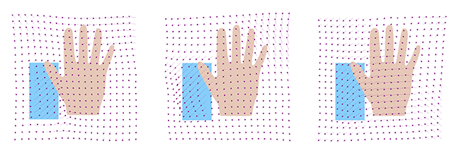^{Figure 1: random samples from a changepoint kernel, where the thumb region (in blue) is modelled differently from the rest of the shape.}

Estimating the Kernel from Example Data

Finally, we show that the kernel (k_s) that arises from estimating the covariance function from observed deformation fields (u_1, ldots, u_n), (u_i : Omega to mathbb{R}^d) is positive-semi definite. Recall from Step 2.4 that this covariance function is defined by

$$k_s(x,x’)=frac{1}{n}sum_{i=1}^n (u_i(x) – overline{u}(x)) (u_i(x’) – overline{u}(x’))^T$$

where

$$overline{u} = frac{1}{n}sum_{i=1}^n u_i.$$

It is easy to see that this is a combination of rule 4 (the part inside the sum), rule 1 (the sum) and rule 2 (the scaling factor (frac{1}{n})).

Hence (k_s) is just a normal, positive semi-definite kernel, which we can in turn combine with any other positive semi-definite kernel using the same rules.