Now that we are able to make a histogram, let’s have a look at what the shape of the histogram is telling us about our data.

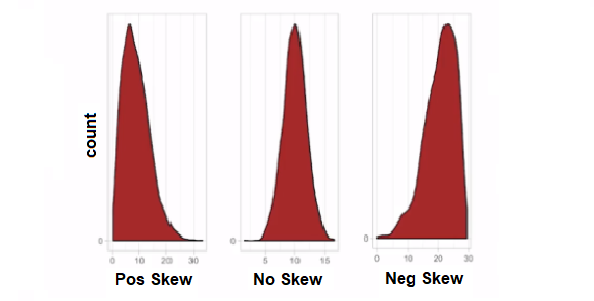
The above image shows three examples of data spread. On the left, the bulk of the data is shifted to the beginning of the graph and has a tail extending to the end of the graph. We refer to this type of distribution as having a positive skew.

The example in the middle has the bulk of the data appearing in the centre of the graph and it looks quite symmetrical. We refer to this type of distribution as having no skew. Another term we use for this type of distribution is bell curve, because it is in the shape of a bell.

In the example on the right, the bulk of the data is shifted to the end of the graph and has a tail extending to the beginning of the graph. We refer to this type of distribution as having a negative skew.

Quantifying Skewness

Skewness is represented as (sk).

For no skew: (sk = 0)
For a negative skew: (sk = -x)
For a positive skew: (sk = +x)

Join the discussion

Do you think that skewness of a histogram will give you a good view of the data set you are working with?

Use the discussion section below and let us know your thoughts. Try to respond to at least one other post and once you’re happy with your contribution, click the Mark as Complete button to check the Step off, then you can move to the next step.