In the previous step, we learned that we can reject the null hypothesis if we can get a small (p)-value. If we are able to reject the null hypothesis, it means that our results are not due to chance, there are real trends, and they’re likely to continue into the future.

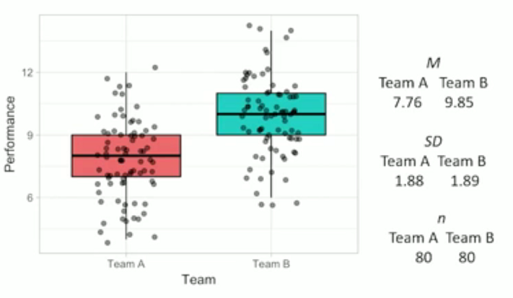
In the above image, we’ve got Team A, with an average of 7.76, and Team B, with an average of 9.85. We’ve also got their standard deviations and we can see that there are 80 people in each team.

We want to find the (p)-value for this comparison.

(P)-values come from things called test statistics or “T-Tests”. A t-test compares 2 groups.

Here’s the formula for performing a t-test:

(t = frac{bar{x}_1 – bar{x}_2}{sqrt{(frac{(hat{sigma_1}^2(n_1 – 1) + hat{sigma_2}^2(n_2 – 1)}{(n_1 – 1)+(n_2 – 1)})(frac{1}{n_1}+ frac{1}{n_2}})})

We have already calculated our means from the previous activities:
(bar{x}_1 = 7,76) and (bar{x}_2 = 9.85)

We have also previously calculated our standard deviations:
({sigma_1}^2 = 3,53) and ({sigma_2}^2 = 3.57)

We also know that our sample size of data is 80 people:
(n_1 = 80) and (n_2 = 80)

Let’s use these numbers now to substitute into our formula:
(t = frac{bar{x}_1 – bar{x}_2}{sqrt{(frac{(hat{sigma_1}^2(n_1 – 1) + hat{sigma_2}^2(n_2 – 1)}{(n_1 – 1)+(n_2 – 1)})(frac{1}{n_1}+ frac{1}{n_2}})})

(therefore t = frac{7,76 – 9,85}{sqrt{(frac{(3,53(80 – 1) + 3,57(80 – 1)}{(80 – 1)+(80 – 1)})(frac{1}{80}+ frac{1}{80}})})

(therefore t = frac{7,76 – 9,85}{sqrt{(frac{(3,53(80 – 1) + 3,57(80 – 1)}{(80 – 1)+(80 – 1)})(frac{1}{80}+ frac{1}{80}})})

(therefore t = frac{-2,09}{sqrt{(frac{(3,53(79) + 3,57(79)}{79+79})(frac{2}{80}})})

(therefore t = frac{-2,09}{sqrt{(frac{(278,87 + 282,03}{158})(frac{2}{80}})})

(therefore t = frac{-2,09}{sqrt{(frac{(560,9}{158})(frac{2}{80}})})

(therefore t = frac{-2,09}{sqrt{(3,55)(0,025)}})

(therefore t = frac{-2,09}{sqrt{0,08875}})

(therefore t = frac{-2,09}{0,298})

(therefore t = -7,013)

In addition to our t-test, we need to calculate the degrees of freedom using this formula:
(df = n_1 + n_2 – 2)
(therefore df = 80 + 80 – 2)
(therefore df = 158)

We can then use these answers to calculate our (p)-value in Excel. We use the absolute value of our t-test score and our degree of freedom in the TDIST formula: =TDIST(ABS(7.013),158.2)

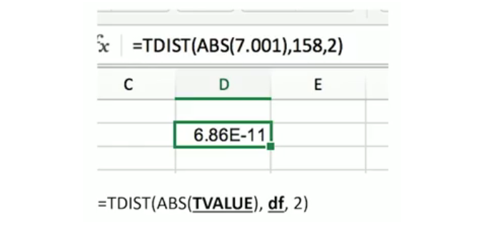
We can see that our result is (6.86 times 10^{-11})
This means that our actual answer is (0.0000000000686)

This tells us that our (p)-value is absolutely tiny.

And our final result is that the likelihood of this scenario happening again is extremely unlikely.

Join the discussion

How does a (p)-value help us to prove or reject a null hypothesis test? Can you share an example?

Use the discussion section below and let us know your thoughts. Try to respond to at least one other post and once you’re happy with your contribution, click the Mark as Complete button to check the Step off, then you can move to the next step.