A closer look at model grids

The video introduced the grid as the mesh of points where a model does its calculations. This visual reading looks more closely at the grid choices a modeller makes – horizontal grids, ways of concentrating resolution, and vertical grids – with real examples of each. Don’t worry about memorising the technical names; focus on the pictures and the idea behind each choice.

Horizontal grids

Horizontal grids define how the continuous ocean surface is divided into a finite set of computational points. There are two broad families – structured grids (regular or curvilinear) and unstructured grids – and the choice affects accuracy, cost, and how well complex coastlines can be represented.

Rectangular longitude-latitude grid

The simplest structured grid uses straight, evenly spaced meridians and parallels. The numerics are straightforward, but its cells shrink strongly toward the poles – which forces very small time steps there and makes this grid unsuitable for global models that include polar regions.

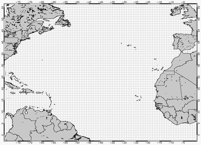Figure 1: A rectangular Lon-Lat grid at large scale, here in the North Atlantic. Image source: oceanmotion.

Curvilinear grids

Curvilinear grids deform the regular grid so that its lines follow smooth paths chosen by the modeller, rather than meridians and parallels. Bipolar and tripolar variants place the “poles” of the coordinate system over land instead of over the ocean, avoiding the polar-convergence problem – now standard practice in global models such as NEMO.

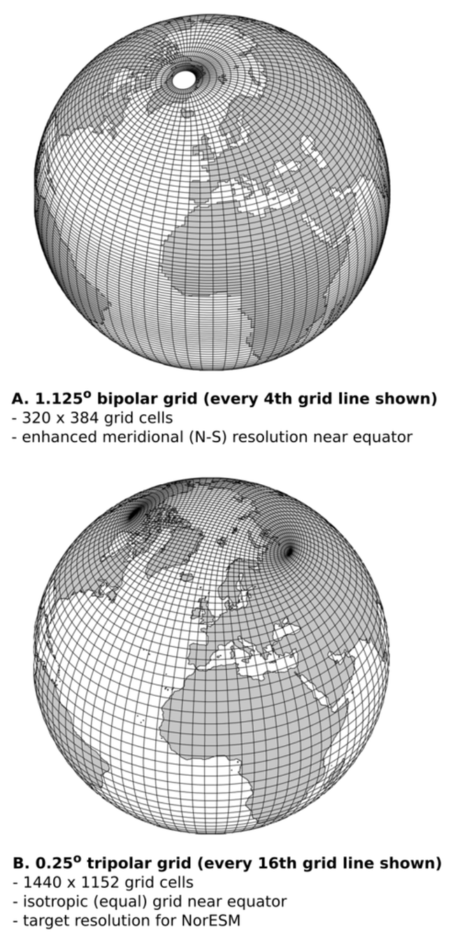Figure 2: Bipolar (left) and tripolar (right) curvilinear grids at global scale. The remaining pole (or poles) sits over the southern continent. Image source: expearth.

Concentrating resolution where it’s needed

Because computational cost grows quickly with the number of grid points, models rarely use fine resolution everywhere. Instead, several strategies concentrate detail only where small-scale processes matter most – near coasts, straits, or energetic regions – while keeping the rest coarser and cheaper.

Swiss-cross refinement

The “Swiss-cross” approach smoothly stretches a structured grid so cells shrink toward a region of interest and grow again away from it, while the grid stays fully structured. This keeps the numerics simple and efficient while still concentrating detail where needed – shown here refined around Iceland.

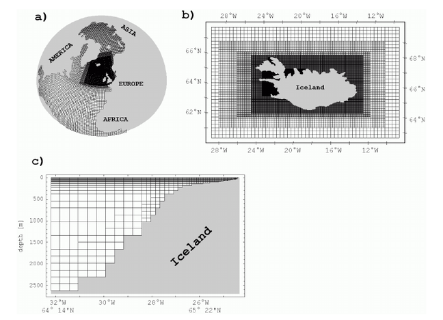Figure 3: An example of Swiss-cross refinement. Source: Logemann and Ingo, 2006.

Unstructured mesh refinement

Because an unstructured mesh is built from independently sized triangles, resolution can vary continuously – coarse triangles far offshore and much smaller ones near the coast, all in one seamless mesh, with no nesting step required.

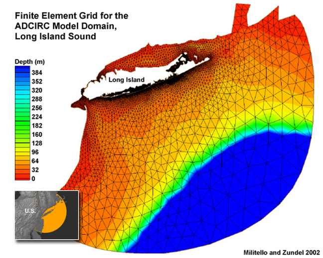Figure 4: An unstructured mesh of triangles (“finite elements”). Triangle size can vary to increase resolution near the coast, where small-scale processes matter, while keeping the open ocean coarse. Image source: COMET Program.

Nesting

Nesting embeds one or more finer “child” grids inside a coarser “parent” grid, letting a regional or coastal model inherit its edges from a larger-scale simulation while resolving local dynamics in far greater detail. In one-way nesting information flows only from parent to child (also called dynamical downscaling); two-way nesting lets the child feed corrections back, at the cost of more complexity.

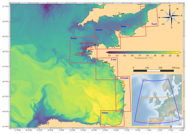Figure 5: A Bay of Biscay configuration with magnified views at 500 m resolution (red), inside a 2.5 km grid (orange), inside a 5 km model (blue). Image source: Petton et al., 2023.

Vertical grids

Beyond the horizontal, a model must also divide the ocean vertically – and this choice strongly affects how well it represents mixing, bottom boundary layers, and how tracers travel. Three main types:

• Z-levels (geopotential): flat layers at fixed depths. Simple and widely used, but they represent steep bottom topography as “steps,” which can create errors
• Terrain-following (sigma): layers that follow the shape of the seafloor, squeezed in shallow water and stretched in deep. Excellent near the bottom and for coastal work, though they can introduce some artificial mixing
• Isopycnic (density-following): layers that follow surfaces of constant density – ideal for tracking how heat, salt, and chemicals move, since in the real ocean they travel mostly along density surfaces, though they struggle where density layers reach the surface in polar regions

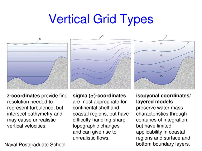Figure 6: Vertical grid types. Horizontal lines mark the water layers as the model sees them: z-levels (fixed depth), sigma (terrain-following), and isopycnic (density-following). Many modern models combine these as hybrid coordinates.

Each of these is a trade-off between accuracy, computational cost, and how faithfully the model captures coastlines, the seabed, and the processes you care about. Keep these grid choices in mind – in the next activities you’ll see how resolution (how fine the grid is) shapes what a model can actually reproduce.