Resolution: how much of the ocean a model can see
In the video, Emanuela Clementi introduced resolution – how finely a model divides space and time. This reading looks closer at what that choice decides, and at the trade-off every modeller must weigh: more detail always costs more computing.
What spatial resolution means
Spatial resolution is simply the size of the grid cells. It sets the smallest feature a model can represent: anything finer than a grid cell is invisible to the model and must be handled indirectly. The range is enormous – from around 100 km for global models down to around 100 m for coastal ones.
Crucially, different jobs need very different resolutions. There is no single “best” value:
| Resolution | Model type | Focus | Constraints |
|---|---|---|---|
| 10-100 km | Global models | Large-scale circulation | Limited detail of small processes |
| 1.5-10 km | Regional models | Basin dynamics; resolve mesoscale eddies | Often nested within global models |
| 100 m-1.5 km | Sub-regional to local | Fine-scale dynamics | Require high-quality boundary conditions |
Adapted from Holt et al. (2025).
Global models prioritise long, stable, multi-decadal runs; coastal models must resolve complex bathymetry and fast local processes. The resolution follows the purpose.
Why resolution decides what a model can see
Resolution is not just a technical setting – it directly controls which physical processes a model can represent explicitly, rather than approximate. The clearest way to appreciate this is to look at the same ocean, simulated at different resolutions. As the grid gets finer, smaller features – fronts, filaments, eddies – progressively appear.
Biological tracers. At coarse resolution (~2°), chlorophyll-a is smeared out, because the fine currents and fronts that structure phytoplankton aren’t resolved. A finer grid (~1/4°) captures these structures – which matters greatly for coastal and shelf regions.
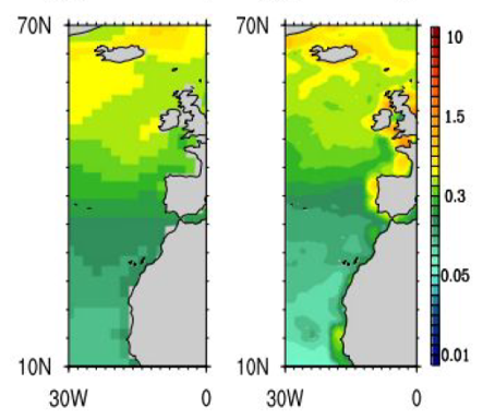
Figure 1: Annual mean chlorophyll-a in the Eastern North Atlantic at 2° (left) and 1/4° (right). The finer model reproduces coastal structure far better. Image source: McKiver et al., 2014.
Sea surface temperature. Temperature fields sharpen dramatically as resolution increases from about 1° down to very fine grids. Coarse runs show smooth, broad gradients; high-resolution runs reveal the fine filaments and fronts made by mesoscale and submesoscale turbulence.
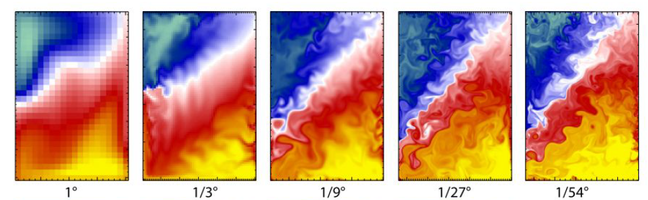
Figure 2: SST simulated at increasing horizontal resolution, from 1° to 1/54°. Image source: Lévy et al., 2012.
Ocean energy (vorticity). Relative vorticity – a measure of local rotation – is especially sensitive to resolution. Models are often classed as eddy-parameterising (~50-100 km), eddy-permitting (~25 km), or eddy-resolving (~10 km or finer); only the finest grids reproduce the sharp, energetic filaments that real eddies generate.
Subsurface structure. The same holds below the surface: temperature anomalies grow richer in detail as resolution increases, because finer grids let the model explicitly generate and carry mesoscale eddies rather than approximate their average effect.
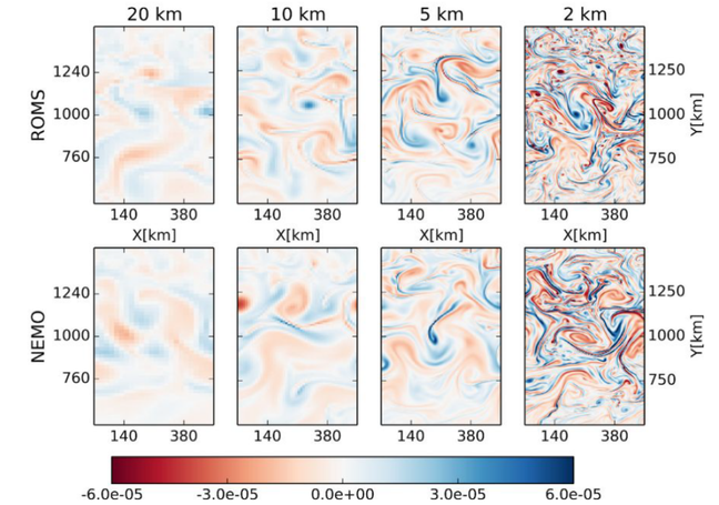
Figure 4: Temperature anomalies at 65 m depth at (a) 3°, (b) 1°, and (c) 1/10° resolution. More features appear as more dynamics are resolved. Image source: Li and Sriver, 2016.
Temporal resolution
Resolution isn’t only about space. The ocean varies across a vast range of timescales – from minutes to millennia. So a model must also step forward in time finely enough to capture the processes that matter: fast processes need a short time step, slow ones can tolerate longer.
The model’s outputs are a separate choice. Results are usually shared as time-averages at selected frequencies – hourly, daily, or monthly being the most common – picked to suit each variable and the purpose of the study.
Space and time are linked
Here’s the key point that ties it together: spatial and temporal resolution cannot be chosen independently. They are bound by the CFL condition – the numerical stability rule that says information in the model must not travel faster than one grid cell per time step.
The consequence is simple but far-reaching: if the grid is fine, the time step must be short. And a shorter time step means many more calculations to simulate the same period. A quick comparison from the lecture makes it vivid: a coastal model with 200 m cells needs a time step under about 3 seconds, while a coarser model resolving ocean eddies with 10 km cells can use a time step of about 100 seconds. Finer in space forces finer in time – and computational cost climbs steeply on both axes at once.
Bridging scales: downscaling
If fine global resolution is too expensive, how do we get local detail? The answer is downscaling: running a coarse global model, then using its output as the boundary conditions for a finer regional or coastal model covering a smaller area. This bridges the global and the local without the impossible cost of running the whole ocean at coastal resolution – and it’s why so many regional systems are “nested” inside global ones.
Key takeaways
- Spatial resolution is the size of the grid cells; it sets the smallest feature a model can see, from ~100 km (global) to ~100 m (coastal)
- Resolution decides which processes are resolved explicitly – finer grids progressively reveal fronts, filaments, and eddies, as the chlorophyll, SST, and vorticity examples show
- Temporal resolution must match the timescales of the processes modelled; outputs are shared as hourly, daily, or monthly averages
- Space and time are linked by the CFL condition: finer grids force shorter time steps, so cost climbs steeply
- Downscaling bridges global and local scales, giving regional detail without running the whole ocean at fine resolution
- Choosing resolution is a key modelling decision – there is no single best value, only the right one for the job and the computing available