Learn more about this course.

Observing long simulations: Sampling distribution of frequencies of 6s

Dr Leonid Bogachev explores what happens when simulating dice rolls looking at sampling distribution of frequencies and the stability of frequencies.

Following from the previous activity on random experiments and samples, let us explore what will happen if we increase the number of simulated instances of 100 rolls of a fair dice.

Repeating the same code as before but with N=500 replicates, and computing the average frequencies of values 1 to 6 over all such simulations, we get

# Set a required number of instances:
N <- 500
# Simulate N runs of 100 dice rolls:
set.seed(2023)
xN <- replicate(N, expr=sample(1:6, size=100, replace=TRUE))
table(xN)/N
## xN
## 1 2 3 4 5 6
## 16.586 16.750 16.870 16.346 16.812 16.636

This time, the average frequencies of all values are more similar to one another!

In particular, the proportion of 6s is now much closer to our expectation of 100/6=16.667.

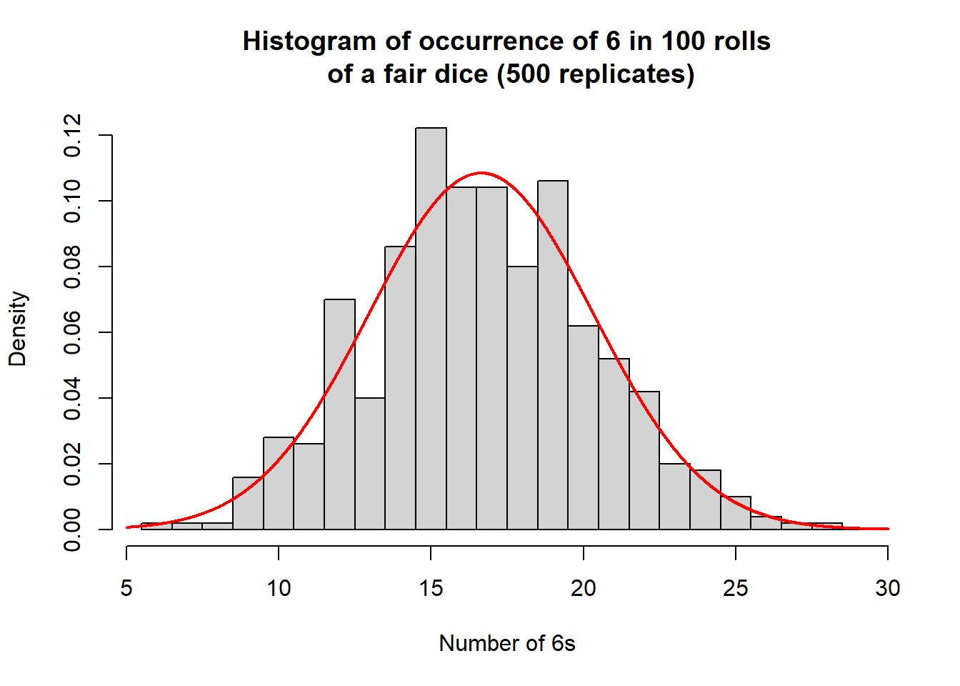
The histogram of observed frequencies of 6 is given in the next image (with the red line showing a normal approximation):

Histogram of occurrence of 6 in 100 rolls of a fair dice, with the normal approximation shown with a curved red line.

The R code used to produce this histogram is as follows:

X6 <- replicate(N, expr=dice6())
hist(X6, freq=FALSE, breaks=0.5+c(5:29), xlab="Number of 6s",
main="Histogram of occurrence of 6 in 100 rollsn
of a fair dice (500 replicates)")
lines(x<-seq(5, 30, 0.01), y=dnorm(x, mean(X6), sd(X6)), col="red", lwd=2)

From the image, we see that the normal approximation works quite well, confirming a bell shape of the simulated data.

A theoretical justification of the normal approximation is based on the so-called central limit theorem, which can be proved mathematically under some reasonable assumptions. This will be explained in more detail later in the course.