
Introduction
So far in the course we have learned how to define a Gaussian Process (GP(mu, k)) by estimating its mean (mu) and covariance function (k) from example data. Estimating the shape variations from normal examples ensures that the model will also only represent anatomically valid shape variations. This type of shape models have been extremely successful in many applications and are by now firmly established.
Estimating the mean and covariance function from example data is only one of many ways to define the parameters of a Gaussian Process.
This week we will look at different choices of the covariance function. We will introduce simple covariance functions in analytic form and discuss how we can build more complex models by combining different covariance functions. By the end of this week, we will see how this idea allows us to define flexible shape models even in cases where only few example shapes are available.
The full potential of modelling shapes using analytically defined Gaussian Processes will become clearer in Week 6, where we will see that these models give rise to powerful methods for establishing correspondence between example shapes.
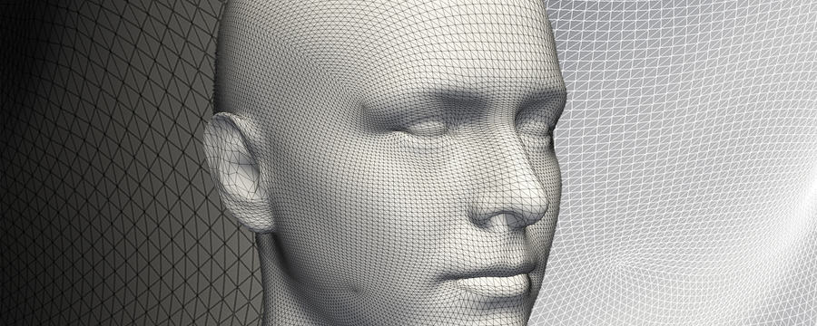
Statistical Shape Modelling: Computing the Human Anatomy

Statistical Shape Modelling: Computing the Human Anatomy
Reach your personal and professional goals
Unlock access to hundreds of expert online courses and degrees from top universities and educators to gain accredited qualifications and professional CV-building certificates.
Join over 18 million learners to launch, switch or build upon your career, all at your own pace, across a wide range of topic areas.


