Shape completion using Gaussian Process regression

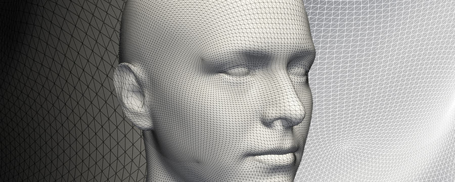
Let’s give Professor Vetter his nose back! Here we see how to apply Gaussian Process regression in Scalismo to retrieve the most fitting nose shape to a face without a nose.

By building a posterior shape model, we not only retrieve the most probable nose, but a whole normal distribution of probable noses all matching the face of the head of our research group, Thomas Vetter.

Each tutorial video is followed by a companion document that you will find in the consecutive Scalismo Lab step.