Skip main navigation

New offer! Get 30% off your first 2 months of Unlimited Monthly. Start your subscription for just £35.99 £24.99. New subscribers only T&Cs apply

Find out more

Fitting models to images

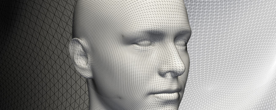
In this video Marcel Lüthi discusses the connection of shape model fitting and segmentation.
6.9
Welcome to week seven. In this last theory video, we’re going to discuss how you can fit a model to an image. With this last tool, you have everything together that you need for developing your own automated system for image analysis. Last week, we have discussed how we can fit a model to a surface. The goal was to find a deformation field that related the reference to the given target surface or contour. Today we’re going to discuss how we can do that for images. The problem is with images, this is going to be much, much harder.
51.9
The reason for that is that if we do a shape fitting, then we already know somehow the target is a shape and we have an explicit representation of it. So we kind of know that our target contour, or surface that we want to explain is a set of points that describe the boundary. If I look at the image instead, I don’t have any boundary information, at least not explicitly. We as human can see it, but in the image, the only thing that I have is the image intensities. So the boundary is only given implicitly.
96.9
The problem of finding this boundary in an image is called the segmentation problem. In its full generality, it can be stated as the problem of partitioning an image into semantically meaningful regions. This is actually a very difficult and still active research problem.
122.2
Now, if you want to fit a model to an image, we somehow also have to solve that segmentation problem. We need to find this boundary. And actually, any successfully-fitted model defines the segmentation. So this tells us something about the difficulty of the task we’re facing. In model fitting, we need to deal with the segmentation problem. But at the same time, we also want that we find correspondence, so that our deformation field maps, for example, the tip of the thumb to the tip of the thumb in the image. So the problem is, in some sense, strictly more difficult than the segmentation problem.
172.6
On the other hand, we have a big advantage, because we don’t want to solve the general segmentation problem. We have prior knowledge. We already know that the object that I want to find, or the boundary of the object that I want to find, is, for example, the hand. And I also have prior knowledge about how hands look like. For example, here, in this illustration, which was a confidence region, I would know that, if a point would end up here in an image, it would be very unlikely to belong to the hand shape. And this encoded prior knowledge, if we make use of it effectively, can actually help and can make it feasible to do model fitting to images.
224.9
It actually turns out that image segmentation is an extremely popular application for shape model. It’s one of the main application areas where shaped models are used for.
242.7
So let’s try to find an algorithm for doing this model fitting to images. Last week, we have discussed the Iterative Closest Point algorithm. This week, we try to adapt it in a way that we can also use it for segmentation. If you remember back, the Iterative Closest Point algorithm was meant as an algorithm for minimising the distance between two point sets or two surfaces, if you will. The first step was, we would find the closest point between the target and the reference. Then we would estimate the transformation based on the corresponding point. In our case, we use the Gaussian Process regression to actually include this prior knowledge about the shape variation of our model.
292.5
And then, we would transform the points after reference such that we are coming closer to the target and repeat the whole procedure.
303.7
Now if you want to at that step for fitting models to images, then it’s actually only step one that doesn’t work anymore. We cannot find closest points because we don’t have an explicit boundary of our object given in the image.
321.6
There is, however, a popular algorithm that already addresses this point. This algorithm is also a classic algorithm. It was proposed in 1995 by Tim Cootes and coworkers. The algorithm is called Active Shape Model fitting. The idea is that we essentially do the same as was in Iterative Closest Point algorithm, but we replace this first step and we don’t try to find the closest point. But we try to find the best matching point, in some sense, that we will have to define.
362.8
Finding this best matching point is in turn divided into two steps. On one hand, we have the modelling step and then we have a search step. In the modelling step, we try to define for each point of the reference somehow, how does the intensity in a neighbourhood look like. So we’re taking somehow a point here of the reference. And then, we could ask the question, if it would be sitting on top of that point, how would the environment look like? So here, for example, if I look in this direction towards the normal of the surface, I would see that I observe, like, dark intensities, so I’m in the background.
414.2
If I go in the other direction, towards the inside, I would see something that represents bone, that has maybe a high intensity. And in this algorithm, the neighbourhood is really often just characterised by a line, which is in normal direction to reference surfaces. Many other types of neighbourhoods would be possible, but this is the most classical one. In the search step, I would then try to find similar neighbourhoods in the image. So if I just consider again the point here, where I know the profile or I know the neighbourhood, how it will look like.
457
If I would then try to take another point, and I would compare the same information, I would find that, if I look in one direction, it’s dark. I would look in the other direction, it’s similarly dark. So a dark intensity. And I could find out, OK that’s not the point that I’m looking for.
480.3
So this is somehow the main idea behind the approach. And now let’s look at the details of the step.
493.5
So in the modelling step, we somehow need to model formally how the intensities look like. The problem with images is if we have two images, they usually look similar, but not the same. There is noise on it, different acquisition devices have different properties. So I cannot just say, I have outside an intensity of 5 and inside an intensity of 200. There’s always certain uncertainty. And the way I deal with it is by modelling the intensities as a normal distribution. So for example, I take a point here where I want to model the intensity. I choose, for example, three points here on that line where I want to formulate the model.
546.2
And then I formulate a normal distribution, which encodes what I assume about intensity values. In this example, we could, for example, say like outside here, at this point, we have a value of 20, signifying that it is background. Here, we’re kind of having self tissue, or skin, that could maybe have a value of 100. And then in the inside, where I have bone, I might have a value of 700. And then to each of these values, I would have a variant. So how much could step intensity actually vary?
587
So I would say, here in the background, I have maybe a low variance, while for the bone, it could be a dense bone or not so dense bony area, and so I could have a large variance.
599.6
And this normal distribution, this could be engineered as I have done it. It could also be learned from examples very similar as we learn a shape model.
613.3
In a second step, the search step, I do what I already outlined a little bit earlier. I would go through the image and I would try to find for any point– So for example, if I’m at this point here and consider just the tip of the thumb, I would go through the image and would try to compare the information that I find in the image with the one that I modelled. And formally, I go through all the points of a neighbourhood around the point where I’m interested in, and compute how likely am I that the information that I find actually matches with my model. And I just choose the point which is most certain.
662.4
So this is what is encoded here, in colour, if I choose the simple intensity model from before. If I’m outside, then I have a very low probability, here encoded by this orange colour. And here, yellow, is also even a lower probability that this point is there. And everything that’s kind of pinkish, here, is around the right point. And my probability would tell me, OK, here it’s quite likely that we’re somehow in the area that you’re looking for. Here you could find this type of information.
703.3
Now, because we have already shape information, we know somehow how the shape can vary. We don’t have to search the whole image for that. We can just compute or search in the neighbourhood of the point that our shape model tells us is still likely that the shape is contained there. So the search can actually be confined to a region around the point, and I know from the shape information how large this region could be, which makes this whole search procedure actually feasible.
738.5
So if you go back to the Active Shape Model fitting algorithm, we have the first step that we have to find the best matching point between the target and the reference. And very similar to the Iterative Closest Point algorithm from last week, these matching points don’t have to be perfect. Because in step two, we’re actually including shape information again, and we perform a Gaussian Process regression using this input as noisy observation. And the result will be corrected by the shape information we have. And by iterating this whole procedure, we hope that we actually get a good fit of the model to the image.
784.2
To summarise, fitting shape models to images is a really difficult problem, because as part of the algorithm, we kind of solve two problems. We find corresponding points, so we would find where is the tip of the thumb in the image. And we find the boundary, so we solve the segmentation problem. To be able to solve both these problems, we need a good shape model and we need an intensity model. Otherwise, this will not be possible. What is nice is that all the concepts that we have discussed for modelling shape can actually be transferred, and we can also use them for modelling intensities.
834.8
We believe that the combination of good shape models, together with good intensity models, makes the automatic analysis of images possible.

As the final step in our exploration of shape models, we show in this video how we can fit a shape model to an image.

We will discuss the segmentation problem and how a successful model fit can be seen as a solution to this problem. Starting from the Iterative Closest Point (ICP) algorithm, we derive a fitting method, which is similar to the famous Active Shape Model (ASM) fitting algorithm.

This article is from the free online

Statistical Shape Modelling: Computing the Human Anatomy

Created by
FutureLearn - Learning For Life

Reach your personal and professional goals

Unlock access to hundreds of expert online courses and degrees from top universities and educators to gain accredited qualifications and professional CV-building certificates.

Join over 18 million learners to launch, switch or build upon your career, all at your own pace, across a wide range of topic areas.

Start Learning now