Data Visualisation with ggplot2: Setting Facets and Scales

Now that we learned how to choose our data, and apply layers of aesthetics and geometries, let’s explore other possible layers of information such as facets and scales.

Good practice

A good practice is to load the packages you need before starting your analysis. It is also recommended to write the packages you need in the script you prepare for a project. This is a list of convenient packages to use with ggplot2:

> library(ggplot2)
> library(RColorBrewer)
> library(viridis)
> install.packages("ggsci")
> library(ggsci)

Note that we need an extra package compared to the previous step.

Setting your working directory in RStudio

Step 1. We recommend that you work in the Project folder Project_Test that we created previously, either by clicking directly on the Project_Test or using the following command

> setwd("/Users/imac/Desktop/exerciseR/Project_Test")
> getwd()
[1] "/Users/imac/Desktop/exerciseR/Project_Test"

Step 2. As a reminder, you can create a specific script file to write your commands and related comments.

Setting Faceting

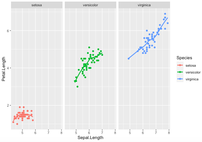
Step 1. Here is an example of how to facet the output by Species, using “facet_wrap()”, that requires the facets argument to be specified, i.e. here the Species

> key <- ggplot(data = iris,aes( x= Sepal.Length,y = 
Petal.Length, color = Species))
> key + geom_point() + geom_smooth(se=FALSE) + 
facet_wrap(~Species)

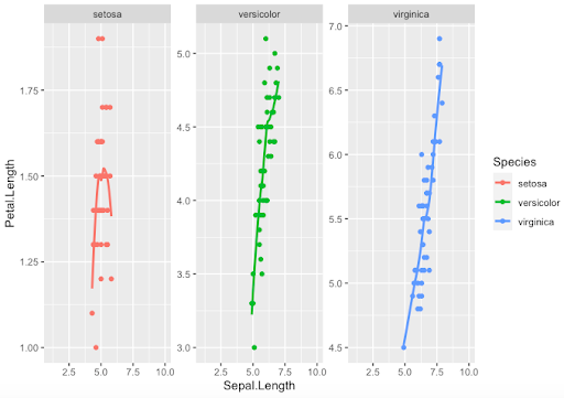
Step 2. Other arguments with “facet_wrap()” give the possibility of fitting the y-axis scales to the values in order to optimize the output

> key + geom_point() + geom_smooth(se=FALSE) + 
facet_wrap(~Species, scale='free_y')

Setting Scales

Scales for positions and axis

Arguments for continuous x and y aesthetics are by default “scale_x_continuous()” and “scale_y_continuous()”. Variants include reversing order or transforming to a log scale. Please see usage in https://ggplot2.tidyverse.org/reference/scale_continuous.html

It is also possible to plot discrete variables using “scale_x_discrete()” or “scale_y_discrete()”

Step 1. To set x-axis limits using “scale_x_continuous()” with limits option

> key + geom_point() + geom_smooth(se=FALSE) + 
facet_wrap(~Species, scale='free_y') + 
scale_x_continuous(limits = c(1, 10))

Step 2. To reverse the x-axis using “scale_x_reverse()”

> key + geom_point() + geom_smooth(se=FALSE) + 
facet_wrap(~Species, scale='free_y') + 
scale_x_reverse()

Scales for colours, sizes and shapes

Continuous colour scales can be specified using many options. Some are already pre-installed in RStudio, such as the RColorBrewer, but other specific colour palettes can be easily installed, loaded and used. Usage for “scale_colour_gradient()” or “scale_fill_gradient()” as examples can be found here https://ggplot2.tidyverse.org/reference/scale_gradient.html

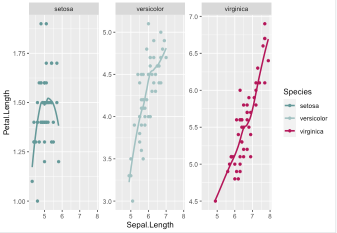
Step 1. Scales can be manually set by choosing specific colours, sizes and shapes

> key + geom_point() + geom_smooth(se=FALSE) + 
facet_wrap(~Species, scale='free_y') + 
scale_shape_manual(values=c(3, 16, 17)) +
scale_size_manual(values=c(2,3,4)) + 
scale_color_manual(values=c('#669999','#a3c2c2', '#b30059'))

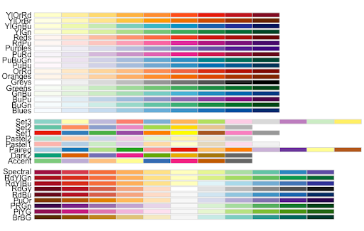
Step 2. Scales can be set using existing colour palettes from the RColorBrewer package

> key + geom_point() + geom_smooth(se=FALSE) + 
facet_wrap(~Species, scale='free_y') + 
scale_color_brewer(palette="RdYlBu")

Note. We use “scale_color_brewer()” to customize colours for lines or points, whereas we would use “scale_fill_brewer()” for filling colours of area, histogram bars, boxplots, etc

Note. RColorBrewer palettes can be consulted with

> display.brewer.all()

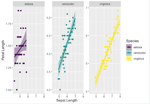
Step 3. Scales can use different options with other color palettes from the viridis package

> new_key <- key + geom_point(aes(color = Species)) + 
geom_smooth(aes(color = Species, fill = Species), method = "lm") + 
facet_wrap(~Species, scale='free_y') 
 
> new_key + scale_shape_manual(values=c(3, 16, 17)) +
scale_size_manual(values=c(2,3,4)) + 
scale_color_viridis(discrete = TRUE, option = "D") + 
scale_fill_viridis(discrete = TRUE)

Note. We changed options for “geom_point()” and “geom_smooth()” to show you some other possible display variations

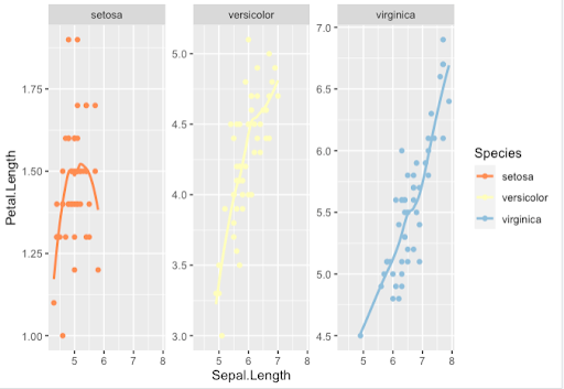
Step 4. Scales can use packages designed to offer color palettes taken from sources such as highly accessed journals. Examples are “scale_color_npg()” (from Nature Publishing Group), “scale_color_lancet()” (from The Lancet journal) or even “scale_color_tron()” (from the film “Tron: Legacy”). Remember that scale_color functions have their scale_fill counterparts

> new_key + scale_color_tron() + scale_fill_tron()

The particular case of missing values

Step 1. Missing values (NA) can exist in any data set, and need to be taken into account when plotting data. Let’s use this very simple data frame containing NA values

• Plotting with default colors in ggplot2. By default, a grey colour will be used for NA

> df_test <- data.frame(x = 1:10, y = 1:10, 
z = c(1, 2, 3, NA, 5, 6, 7, NA, 8, NA))
> plot_test <- ggplot(df_test, aes(x, y)) + 
geom_tile(aes(fill = z), size = 10)
> plot_test

• We can ask to have no colour of NA values

> plot_test + scale_fill_gradient(na.value = NA)

• Or color NA values in a chosen colour, such as “red3” here

> plot_test + scale_fill_gradient(na.value = "red3")

• Or use another colour palette, instead of default ggplot2 colours, and you will still be able to specify the NA values. Because we need many colors in this palette we use “scale_fill_gradientn()” instead of “scale_fill_gradient()”

> plot_test + scale_fill_gradientn(colours = viridis(7), na.value = "white")