Data Visualisation with ggplot2: Setting Themes, Coordinates and Labels

Data Visualisation in RStudio – other possible layers of information such as facets and scales

Introduction

Now that we learned how to choose our data, and apply layers of aesthetics and geometries, let’s explore other possible layers of information such as facets and scales.

Good practice

> library(ggplot2)
> library(RColorBrewer)
> library(viridis)
> library(ggsci)

Setting your working directory in RStudio

Step 1. We recommend you to work in the Project folder Project_Test that we created previously, either by clicking directly on the Project_Test or using the following command

> setwd("/Users/imac/Desktop/exerciseR/Project_Test")
> getwd()
[1] "/Users/imac/Desktop/exerciseR/Project_Test"

Step 2. As a reminder, you can create a specific script file to write your commands and related comments.

Setting Themes

Themes encompass options for the general graphical display of a graph, by modifying non-data output such as the legends, the panel background, etc… You can refer to “theme()” usage including examples in
https://www.rdocumentation.org/packages/ggplot2/versions/3.3.3/topics/theme

Step 1. We will use the same new_key variable that we created in the previous Step

> new_key <- key + geom_point(aes(color = Species)) + 
geom_smooth(aes(color = Species, fill = Species), 
method = "lm") + facet_wrap(~Species, scale='free_y') 
> new_key + scale_color_tron() + scale_fill_tron()

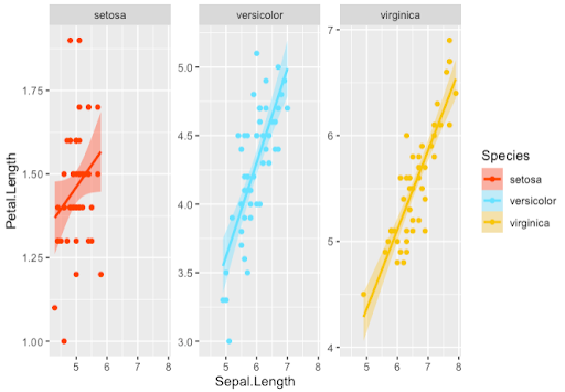
Step 2. By default the themes are set to “theme_grey()” (or gray). The same previous output will be displayed if you type:

> new_key + scale_color_tron() + scale_fill_tron() + theme_grey()

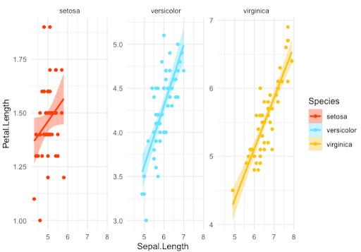
Step 3. Don’t forget that, as for other functions, you can learn about other variants and options of themes while typing the command in RStudio. If not, simply start typing the function and hit the TAB button on your keyboard. Here is different theme:

> new_key + scale_color_tron() + scale_fill_tron() + theme_minimal() 

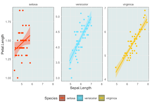
Step 4. You can now customize the background color, and also set the legends positions. Here is an example on how to place the legend at the bottom.

> new_key + scale_color_tron() + scale_fill_tron() + 
theme_minimal() + theme(legend.position = "bottom", 
panel.background = element_rect(fill = "#e0ebeb"), 
legend.key = element_rect(fill = "#669999"))

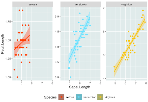
Step 5. Note the difference hereafter if when we leave the default theme (just by removing “theme_minimal()” to come back to basic)

> new_key + scale_color_tron() + scale_fill_tron() + 
theme(legend.position = "bottom", panel.background = 
element_rect(fill = "#e0ebeb"), 
legend.key = element_rect(fill = "#669999"))

Step 6. It is also possible to customize the position or justification of your legend. To do this, you can use “theme_position()” to set the position in the whole panel, and “theme_justification()” to set the position in the legend area. They are defined with a vector of length 2, indicating x and y positions in terms of space coordinates, where c(1, 0) is the bottom-right position

> new_key + scale_color_tron() + scale_fill_tron() + 
theme(legend.position=c(1,0), legend.justification = c(1, 0))

Setting Coordinates

The coordinate system controls the position of objects into the main panel, as well as axis and grid lines display. The most classically used are cartesian coordinates, but many other exist

Step 1. Let’s start with “coord_cartesian()” which is set by default. The following commands will have the same output

> new_key + scale_color_tron() + scale_fill_tron()
> new_key + scale_color_tron() + scale_fill_tron() 
+ coord_cartesian()

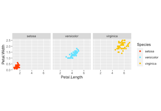
Step 2. We are now used to see specific options with each function. Let’s fix a ratio from x to y axis, and see how this affects the display in the main panel

> new_key2 <- ggplot(data = iris) + geom_point(aes(x = 
Petal.Length, y = Petal.Width, color = Species)) + 
facet_wrap(~Species) + scale_color_tron() + scale_fill_tron()
 
> new_key2 + coord_fixed(ratio = 2)

Note. The panel borders colored in grey show you the new display

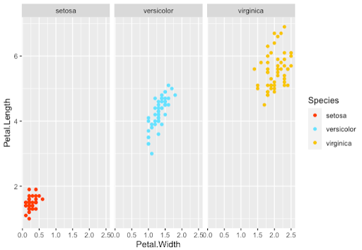
Step 3. A logarithmic transformation can be applied to x and y-axis

> new_key2 + coord_trans(x = "log2", y = "log2")

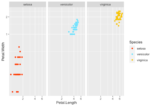
Step 4. It also possible to swap x-axis values to y-axis and vice-versa

> new_key2 + coord_flip()

Step 5. Compare these 2 outputs to see how it changes the display for other plot types

• Barplot

> new_key3 <- ggplot(iris, aes(x=Petal.Length, Petal.Width)) 
+ geom_bar(stat="identity", fill="white", color="red3")
> new_key3

• Right Barplot

> new_key3 + coord_flip()

Setting Labels

The Labs or Labels system controls the legend, axis and plot labels. You can find examples and usage here https://ggplot2.tidyverse.org/reference/labs.html

Step 1. Let’s start with default “labs()” to set the legend title. The following commands will have the same output

> new_key + scale_color_tron() + scale_fill_tron()
> new_key + scale_color_tron() + scale_fill_tron() 
+ labs(color = "Species")

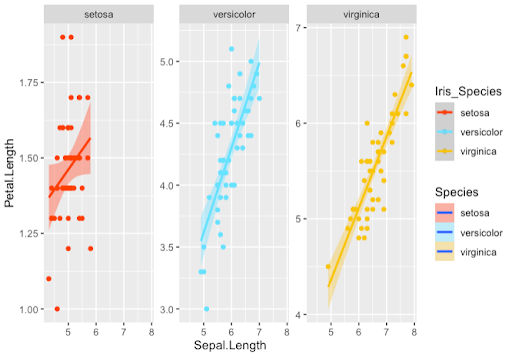
Step 2. Notice how we modify the legend title by:

> new_key + scale_color_tron() + scale_fill_tron() + 
labs(color = "Iris_Species")

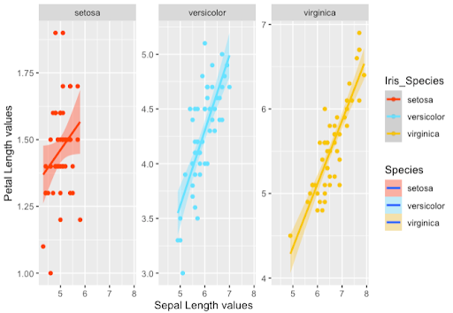
Step 3. To modify also the x-axis and y-axis names

> new_key + scale_color_tron() + scale_fill_tron() + 
labs(color = "Iris_Species", x = "Sepal Length values", 
y = "Petal Length values")

Step 4. Note that it might often be possible to do the same thing using different functions or options. Let’s see 2 options to add a title

> new_key + scale_color_tron() + scale_fill_tron() + 
labs(color = "Iris_Species", x = "Sepal Length values", 
y = "Petal Length values", title = "Petal vs. Sepal Legnth")

 
> new_key + scale_color_tron() + scale_fill_tron() + 
labs(color = "Iris_Species", x = "Sepal Length values", 
y = "Petal Length values") + ggtitle("Petal vs. Sepal Legnth")