
Landsat 8 & 9 imagery in QGIS
Now that you have your satellite imagery, let’s get it into QGIS!
Adding our image to QGIS
Before we open our imagery in QGIS we will need to extract it.
Extracting our imagery
Your image files are packaged into a special .tar format. This is fairly similar to a zip file.
You may need extra software to open it if your computer doesn’t recognise tar files. We recommend 7-Zip, which is free and can be downloaded here. Do make sure that you download the correct version of 7-Zip for your computer!
The exact method will vary depending on which software you are using, but with 7-Zip:
- 1) Right-click your tar file and select “7-Zip” and then “Extract to “LC09L1TP…””
 Extracting our data.
- 2) When this has finished running, open your new folder – you should have 24 different files.
You can view a preview of your image by double-clicking the “…thumb_large.jpeg” or “…thumb_small.jpeg”.
 Extracted Landsat data, including thumbnails.
Most of these files are the different bands of the satellite image – you can spot these as they end in B “…B[number].TIF” (with B standing for ‘Band’). There is also metadata (information about the image) and other files too.
Adding our bands to QGIS
Now we are finally ready to start viewing our satellite imagery!
- 1) Open QGIS. Start a new project if you like, otherwise open your old one.
- 2) On the Main Menu select Layer > Add Layer > Add Raster Layer.
- 3) Click the browse button and find your Landsat folder.
- 4) Change File Type to GeoTIFF.
- 5) Hold down the Ctrl key on your keyboard and select all the TIFF files with a “B” near the end – there should be 11 in total!
- 6) Click the Open button, and then Add, and Close.
 Change the filetype to GeoTIFF and selecting all 11 Landsat bands.
You should have eleven new images in you Layers Panel – have a go at turning the top layers off to view the ones beneath and compare them in the Map Window. What is similar and what is different about them?
 Viewing our 11 Landsat bands.
Creating a composite
Individually these bands are not that much use! We want to be able to create different RGB composites in colour using combinations of different bands. To do this we are going to merge all our data together into a single raster layer.
- 1) On the main menu go to Raster > Miscellaneous > Build Virtual Raster
Virtual Rasters are a quick way of combining different bands together without creating massive new files. They work best if you are keeping all your data on a single computer and not sharing it with lots of different people.
- 2) Click the Browse button and then click the Select All.
- 3) Make sure the bands are in numerical order – you will probably have to drag B10 and B11 to the bottom of the list.
 Selecting and correctly ordering our Landsat bands.
- 4) Tick “Place each input file into a separate band”.
- 5) Click the Browse button to the right of the Virtual field and click Save to File.
- 6) In your Landsat folder, type “landsat_composite” for your filename and click Save.
- 7) Finally click Run and Close when it has finished!
 Building our Landsat composite as a virtual raster.
 Our Landsat colour composite layer.
Changing the bands
 Landsat 8 & 9 bands. Based on an image courtesy of NASA.
- 1) In the Layers Panel right-click the “landsat_composite” layer and select Properties.
- 2) Change “Red band” to Band 04, “Green band” to Band 03, and “Blue Band” to Band 02.
- 3) Click OK.
 Setting our RBG bands to 4/3/2.
 Our true colour Landsat composite – notice the labels beside the RGB bands in the Layers Panel.
Band combinations
 Landsat 8 & 9 and Sentinel-2 band comparison. Based on image courtesy of NASA.
| composite | bands | uses |
|---|---|---|
| true colour | 4/3/2 | realistic colours, like the naked eye |
| natural-like | 7/5/3 | quite realistic but exaggerated colours |
| false colour infrared | 5/4/3 | shows vegetation in red |
| false colour urban | 7/6/4 | shows built-up areas in purple |
| false colour agriculture | 6/5/2 | shows healthy plants in bright green |
| false colour land/water | 5/6/4 | studying wetland environments |
| false colour shortwave infrared | 7/5/4 | like 7/5/3 |
| false colour geology 1 | 7/6/2 | studying the geological landscape |
| false colour geology 2 | 6/3/2 | studying the geological landscape |
Changing the band combination
- 1) In the Layers Panel right-click the “landsat_composite” layer and select Properties.
- 2) Change “Red band” to the first number of your chosen combination (e.g. for 5/4/3, change it to 5).
- 3) Change “Green band” to the second number.
- 4) Change “Blue band to the third.
- 5) Click OK.
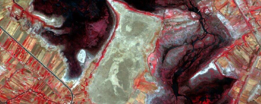
 A 5/4/3 false colour composite showing the expanding farmland in red.
How does the Landsat imagery of your area of interest compare to the Sentinel-2 we downloaded last week?
Advanced Archaeological Remote Sensing: Site Prospection, Landscape Archaeology and Heritage Protection in the Middle East and North Africa

Advanced Archaeological Remote Sensing: Site Prospection, Landscape Archaeology and Heritage Protection in the Middle East and North Africa
Reach your personal and professional goals
Unlock access to hundreds of expert online courses and degrees from top universities and educators to gain accredited qualifications and professional CV-building certificates.
Join over 18 million learners to launch, switch or build upon your career, all at your own pace, across a wide range of topic areas.


