An introduction to layouts using Python

What are layouts?

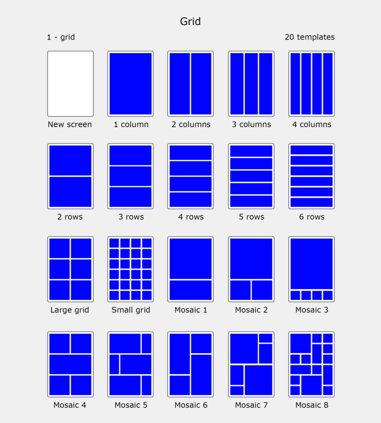
The layout provides meaning to your design and makes it look noticeably appealing. It helps to maintain balance from page to page. Grids are an essential component of the layout design, as they support all layouts, infographics, and presentations incredibly well.

Layout design comprises one grid or a group of grids, depending on the requirements.

Click to enlarge

So far, we have only shown one figure at a time with Bokeh. However, we can use custom layouts to group them into rows and / or columns.

Previously in Matplotlib, you generated the number of rows and columns when you first drew the figure and axes. However, with Bokeh, you start with plots and then choose how they are to be laid out when displayed. In this step, we will use Bokeh in Python and see examples as demonstrations of how to layout plots using rows and columns.

Creating rows and columns

To start with, let us try laying out plots in a single row with multiple columns, using the row function. This is imported from bokeh.layouts.

Demonstration: Single row with multiple columns

Step 1

Import figure from Bokeh layouts.

Code:

from bokeh.plotting import figure, output_notebook, show
from bokeh.layouts import row
output_notebook()
figure_width = 300
figure_height = 400

Output:

BokehJS 2.2.3 successfully loaded

Step 2

Select multiple arguments (one or more plots or other layouts) to arrange into a row.

Code:

square_plot = figure(plot_width=figure_width, plot_height=figure_height)
circle_plot = figure(plot_width=figure_width, plot_height=figure_height)
triangle_plot = figure(plot_width=figure_width, plot_height=figure_height)

square_plot.square([0], [0], size=20)
circle_plot.circle([1], [1], size=30)
triangle_plot.triangle([2], [2], size=30)

Step 3

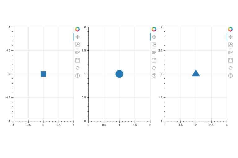
Arrange them into a single row using the row function.

Code:

r1 = row(square_plot, circle_plot, triangle_plot)
show(r1)

Output:

Click to enlarge

Like rows, there are also columns, which are created the same way but which lay out the data in a single column with multiple rows.

Demonstration: Single column with multiple rows

Step 1

Import figure from Bokeh layouts.

Code:

from bokeh.layouts import column

Arrange them into a single column using the column function.

Code:

c1 = column(square_plot, circle_plot, triangle_plot)
show(c1)

Output:

Did you get an output where multiple rows are seen, one below the other, in a single column?

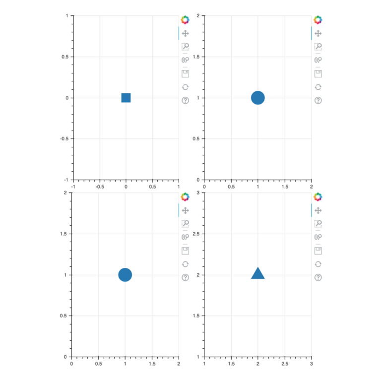
Demonstration: Single two-column layout with two rows

Since we already have a plot ready, just arrange them into a single two-column layout with two rows.

Code:

c2 = column(row(square_plot, circle_plot), row(circle_plot, triangle_plot))
show(c2)

Output:

Click to enlarge

Gridplot layout

An alternative method to making grid plots is to use the gridplot layout function. In the previous operations, row and column used the sizes of the individual plots whereas the gridplot function allows overriding of these sizes with the use of the plot_width and plot_height keyword arguments, applying the sizes to each of the plots.

Demonstration: Gridplot layout

Step 1

Import gridplot from Bokeh layouts.

Code:

~~ python
from bokeh.layouts import gridplot
~~~

Step 2

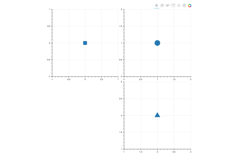
Draw the plots into a two-by-two grid, fixing each plot’s size to 400 by 400. Leave a space in the bottom right plot.

Code:

g1 = gridplot([
 [square_plot, circle_plot], 
 [None, triangle_plot]
 ], 
 plot_width=400, 
 plot_height=400
)
show(g1)

Output:

Click to enlarge

Moving on, we will explore some attractive advanced layouts and sizing options. To learn more about layouts in Bokeh, read the resource provided below.

Read: Creating Layouts [1]

References

1. Creating Layouts [Document]. Bokeh; [date unknown]. Available from: https://docs.bokeh.org/en/latest/docs/user_guide/layout.html#userguide-layout