Visual profiling and tracing of the GPU codes

In this step, we will present some tools for visual profiling and tracing of the GPU codes. These tools are generally available with the GPU SDK, some of them can also be installed separately. The tools can’t be invoked through Jupyter notebooks directly, but you can try them if you have access to a system with direct command-line or GUI execution. Profiling and tracing are useful in terms of code performance analysis and hints at optimization.

Tools capable of profiling and/or tracing CUDA and OpenCL codes:

CUDA:

• nvprof: command line profiling tool from CUDA toolkit (deprecated in CUDA 11)
• nvvp: visual profiler (GUI) tool from CUDA toolkit (deprecated in CUDA 11)
• Nvidia Nsight Systems
• TAU (Tuning and Analysis Utilities): open source tool for profiling and tracing
• other tools: Vampir, Scalasca (for large scale applications)…

OpenCL:

• on NVIDIA cards: OpenCL profiling not supported since CUDA 8
• on AMD cards: OpenCL profiling with Radeon GPU profiler
• TAU (Tuning and Analysis Utilities): open source tool for profiling and tracing
• other tools: Vampir, Intel VTune Profiler…

Profiling and tracing of CUDA codes

You already know how to use the profiling tool nvprof, e.g., for the CUDA Riemann sum code with two kernels

$ nvprof ./riemann_cuda_double_reduce

you obtained the following output in command line (see the previous step Profiling of the Riemann sum codes with two GPU kernels):

==2194== NVPROF is profiling process 2194, command: ./riemann_cuda_double_reduce
Found GPU 'Tesla K80' with 11.173 GB of global memory, max 1024 threads per block, and 13 multiprocessors
CUDA kernel 'medianTrapezium' launch with 976563 blocks of 1024 threads
CUDA kernel 'reducerSum' launch with 1 blocks of 1024 threads

Riemann sum CUDA (double precision) for N = 1000000000 : 0.34134474606854243
Total time (measured by CPU) : 2.130000 s
==2194== Profiling application: ./riemann_cuda_double_reduce
==2194== Profiling result:
 Type Time(%) Time Calls Avg Min Max Name
 GPU activities: 79.45% 668.84ms 1 668.84ms 668.84ms 668.84ms reducerSum(double*, double*, int, int)
 20.55% 172.96ms 1 172.96ms 172.96ms 172.96ms medianTrapezium(double*, int)
 0.00% 8.4480us 1 8.4480us 8.4480us 8.4480us [CUDA memcpy DtoH]
 API calls: 46.26% 1.01224s 3 337.41ms 10.109us 1.00527s cudaFree
 38.47% 841.87ms 1 841.87ms 841.87ms 841.87ms cudaMemcpy
 14.56% 318.66ms 2 159.33ms 587.33us 318.07ms cudaMalloc
 0.34% 7.3509ms 582 12.630us 305ns 476.82us cuDeviceGetAttribute
 0.27% 6.0104ms 6 1.0017ms 998.14us 1.0108ms cuDeviceTotalMem
 0.05% 1.1714ms 1 1.1714ms 1.1714ms 1.1714ms cudaGetDeviceProperties
 0.03% 589.12us 6 98.187us 95.529us 103.46us cuDeviceGetName
 0.01% 267.51us 2 133.76us 23.377us 244.14us cudaLaunchKernel
 0.00% 31.279us 6 5.2130us 2.8280us 15.291us cuDeviceGetPCIBusId
 0.00% 10.163us 1 10.163us 10.163us 10.163us cudaSetDevice
 0.00% 6.6350us 12 552ns 392ns 1.2660us cuDeviceGet
 0.00% 3.6970us 3 1.2320us 417ns 2.0400us cuDeviceGetCount
 0.00% 2.4670us 6 411ns 357ns 584ns cuDeviceGetUuid

Tracing can be done with nvvp, e.g., for the CUDA Riemann sum code with two kernels:

$ nvvp ./riemann_cuda_double_reduce

Visual profiling can be invoked with many options for analysis of the CUDA code. The picture below shows the traces for the Riemann sum code with two kernels and the summary of both kernels execution (average duration, FLOP, multiprocessor occupancy…).

(Click to expand)

One can observe from the traces that the kernel reducerSum is executed after the kernel medianTrapezium and that for the latter 91.1% Streaming Multiprocessor (SM) occupancy was achieved with 86000005646 Double Precision Floating Point Operations (Flop) in 172.91868 milliseconds. For the kernels, the parameters can be shown graphically, e.g., the performance in Flops. You can calculate the latter yourself from data in the summary, e.g., for the kernel medianTrapezium:

86000005646/172.91868*1000/10^9 = 497.34 GFlops

You can then compare this performance to the theoretical FP64 (double) performance of 1371 GFlops for the Tesla K80 GPU (on which the CUDA program was executed) and determine the efficacy of the code.

As already pointed out, the tools nvprof and nvvp are already deprecated in CUDA 11 and will be discontinued. They are replaced by Nvidia Nsight Systems. The equivalent of nvprof in the command line is nsys. One can profile the CUDA Riemann sum code with two kernels in the following way:

$ nsys profile --trace cuda ./riemann_cuda_double_reduce
$ nsys stats report1.qdrep

First, we generate the profiling report report1.qdrep of which the output can be subsequently invoked in the command line by the nsys stats call:

 Time(%) Total Time (ns) Num Calls Average Minimum Maximum Name
 ------- --------------- --------- ------------- ----------- ----------- ----------------
 79.7 614,696,365 1 614,696,365.0 614,696,365 614,696,365 cudaMemcpy
 19.5 150,392,555 2 75,196,277.5 170,492 150,222,063 cudaMalloc
 0.8 5,854,639 3 1,951,546.3 2,800 5,766,738 cudaFree
 0.0 41,361 2 20,680.5 7,670 33,691 cudaLaunchKernel


 Time(%) Total Time (ns) Instances Average Minimum Maximum Name
 ------- --------------- --------- ------------- ----------- ----------- --------------------------------------
 96.7 594,399,821 1 594,399,821.0 594,399,821 594,399,821 reducerSum(double*, double*, int, int)
 3.3 20,265,788 1 20,265,788.0 20,265,788 20,265,788 medianTrapezium(double*, int)


 Time(%) Total Time (ns) Operations Average Minimum Maximum Operation
 ------- --------------- ---------- ------- ------- ------- ------------------
 100.0 3,040 1 3,040.0 3,040 3,040 [CUDA memcpy DtoH]

The equivalent of nvvp is nsys-ui. By typing in the command line

$ nsys-ui

the Nsight Systems GUI will be invoked. One can then load the previously generated report report1.qdrep to visualize traces. The picture below shows the traces for the Riemann sum code with two kernels visualized by the Nsight Systems GUI.

(Click to expand)

Profiling and tracing of OpenCL codes

For profiling and tracing OpenCL codes, one can use the TAU Performance System. Unfortunately, it is not a part of GPU SDKs, therefore it must be installed separately.

Profiling of the OpenCL Riemann sum code with two kernels can be done with TAU in the following way. First, we generate profiles with:

$ tau_exec -T serial -opencl ./riemann_opencl_double_reduce

This will generate 2 profile files: profile.0.0.0 and profile.0.0.1.

Profiling in command line can be done with:

$ pprof

The output is a detailed profiling report, we will show just an excerpt from it:

NODE 0;CONTEXT 0;THREAD 1:
---------------------------------------------------------------------------------------
%Time Exclusive Inclusive #Call #Subrs Inclusive Name
 msec total msec usec/call
---------------------------------------------------------------------------------------
100.0 0.0165 767 1 3 767448 .TAU application
 75.3 577 577 1 0 577820 reducerSum
 24.7 189 189 1 0 189608 medianTrapezium
 0.0 0.00275 0.00275 1 0 3 ReadBuffer

FUNCTION SUMMARY (total):
---------------------------------------------------------------------------------------
%Time Exclusive Inclusive #Call #Subrs Inclusive Name
 msec total msec usec/call
---------------------------------------------------------------------------------------
100.0 20 2,035 2 34 1017668 .TAU application
 37.6 766 766 1 0 766036 cl_int clEnqueueReadBuffer(cl_command_queue, cl_mem, cl_bool, size_t, size_t, void *, cl_uint, const cl_event *, cl_event *) C
 28.4 577 577 1 0 577820 reducerSum
 12.7 258 258 1 0 258078 cl_int clBuildProgram(cl_program, cl_uint, const cl_device_id *, const char *, void (*)(cl_program, void *), void *) C
 9.3 189 189 1 0 189608 medianTrapezium
 7.9 160 160 1 0 160755 cl_context clCreateContext(const cl_context_properties *, cl_uint, const cl_device_id *, void (*)(const char *, const void *, size_t, void *), void *, cl_int *) C
 2.0 41 41 1 0 41175 cl_int clGetPlatformIDs(cl_uint, cl_platform_id *, cl_uint *) C
 1.0 21 21 2 0 10596 cl_int clEnqueueNDRangeKernel(cl_command_queue, cl_kernel, cl_uint, const size_t *, const size_t *, const size_t *, cl_uint, const cl_event *, cl_event *) C
 0.0 0.279 0.279 1 0 279 cl_int clReleaseProgram(cl_program) C
 0.0 0.025 0.025 2 0 12 cl_kernel clCreateKernel(cl_program, const char *, cl_int *) C
 0.0 0.024 0.024 1 0 24 cl_command_queue clCreateCommandQueue(cl_context, cl_device_id, cl_command_queue_properties, cl_int *) C
 0.0 0.011 0.011 2 0 6 cl_int clReleaseKernel(cl_kernel) C
 0.0 0.011 0.011 2 0 6 cl_mem clCreateBuffer(cl_context, cl_mem_flags, size_t, void *, cl_int *) C
 0.0 0.01 0.01 1 0 10 cl_int clFlush(cl_command_queue) C
 0.0 0.009 0.009 1 0 9 cl_program clCreateProgramWithSource(cl_context, cl_uint, const char **, const size_t *, cl_int *) C
 0.0 0.006 0.006 1 0 6 cl_int clReleaseCommandQueue(cl_command_queue) C
 0.0 0.006 0.006 7 0 1 cl_int clSetKernelArg(cl_kernel, cl_uint, size_t, const void *) C
 0.0 0.004 0.004 1 0 4 cl_int clFinish(cl_command_queue) C
 0.0 0.004 0.004 2 0 2 cl_int clGetKernelInfo(cl_kernel, cl_kernel_info, size_t, void *, size_t *) C
 0.0 0.003 0.003 1 0 3 cl_int clReleaseContext(cl_context) C
 0.0 0.00275 0.00275 1 0 3 ReadBuffer
 0.0 0.002 0.002 1 0 2 cl_int clGetDeviceIDs(cl_platform_id, cl_device_type, cl_uint, cl_device_id *, cl_uint *) C
 0.0 0.001 0.001 2 0 0 cl_int clGetCommandQueueInfo(cl_command_queue, cl_command_queue_info, size_t, void *, size_t *) C

The GUI profiling utility can be invoked with:

$ paraprof

The visualisation of profiles (threads), i.e., one profile for OpenCL API calls and the other for OpenCL kernels, can be seen on the pictures below.

(Click to expand)

(Click to expand)

Tracing of the OpenCL Riemann sum code with two kernels can be done with TAU in the following way. Again, we first generate traces (tautrace.0.0.0.trc and tautrace.0.0.1.trc) with:

$ TAU_TRACE=1 tau_exec -T serial -opencl ./riemann_opencl_double_reduce

Then we can use the jumpshot utility within TAU to visualize the traces:

$ tau_treemerge.pl
$ tau2slog2 tau.trc tau.edf -o tau.slog2
$ jumpshot tau.slog2

On the pictures below you can see the traces with the description legend.

(Click to expand)

(Click to expand)

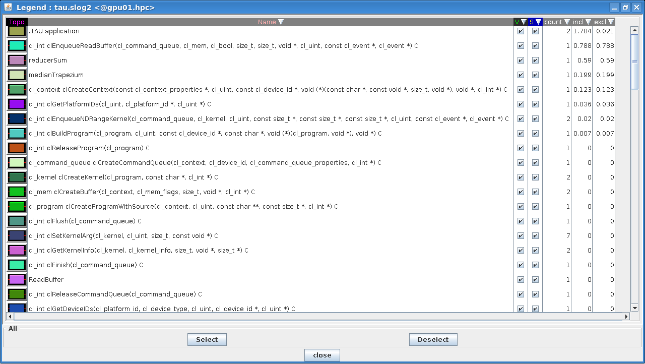
The second trace (thread 1) shows the OpenCL kernels on a timeline: it is evident that the reducerSum kernel is executed after the medianTrapezium kernel, as is the case of the trace showing CUDA kernels.

The latter observation should be clarified in some detail. In CUDA all operations executed on the device belong to the so-called default stream. Multiple kernels submitted to the same stream are executed consequently one after another. If one needs concurrent execution of multiple kernels, then every kernel must be defined in a different stream. For synchronization of kernels execution, one can use cudaDeviceSynchronize(), which is in fact a blocking call, i.e., it blocks any further execution until the device (GPU) has finished all the tasks launched to that point.

Similarly, multiple OpenCL kernels enqueued in the same command queue are executed consequently one after another. Concurrent execution of multiple kernels is achieved by creating multiple command queues.