Noise and noise reduction using filtering

Image noise is a common problem you may encounter when preparing images for analysis. The type of noise you will encounter will depend on the type and quality of your photographic equipment. This article supports the previous videos by describing some common types of noise, and how the noise can be reduced by using filters.

Gaussian noise

Every pixel in an image is a measure of light hitting the sensor of the camera at an exact point in space and time when the image is taken. However, the precision of the sensors may not be perfect, meaning that the recorded pixel value is not the same as the ‘true’ value at that point. We assume that the recorded values of each pixel are most likely to be at or near the true pixel value, and increasingly unlikely to take values further away from the true value. This can be modelled as a Gaussian (or normal) probability distribution with the mean value (mu) as the true pixel value and the standard deviation (sigma) representing the spread of the measurement errors around this mean. The figure below shows the characteristic bell shape of the Gaussian probability density function (PDF) labelled P(X), and some simulated noise of increasing intensity on the same example image.

Uniform noise

While most image data is likely to suffer from Gaussian noise to a greater or lesser degree, in some contexts the primary source of noise is what is known as uniform noise. In this case the measured pixel values are equally likely to be spread across a range of possible values either side of the true value. Here the PDF of the recorded value of each pixel value takes the form of a rectangle either side of the true value (shown as zero in the chart below), with the spread of the noise denoted as (a).

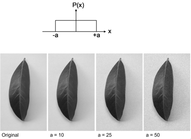
Uniform noise is commonly found in the case of poor lighting where the sensitivity of the sensor is such that is becomes harder to correctly measure the amount of light with great accuracy.

Salt and pepper noise

The final kind of noise we will mention in salt and pepper noise. This is so-called because it appears as white or black specks in the image, where individual pixels have taken saturated maximum (white) or minimum (values). Generally, this is caused by faults in the image sensor itself, and in fact many modern cameras are calibrated to correct for such errors. If you do think your images are suffering from this type of noise however, a good way to check is to look at the image histogram and check for any spikes at the top or bottom of the intensity range.

Reducing noise

Noise cannot be eliminated after image acquisition, but there are ways to reduce it using filtering. The type of filter used will vary depending on the type of noise in the image, but the basic principle is the same:

• For every pixel we consider a window or kernel of surrounding pixels. This is often just the immediately adjacent pixels (a 3 x 3 kernel), but 5 x 5 kernels are or even larger can be used.
• For this subset of pixels (9 pixels in the case of a 3 x 3 kernel) some statistical calculation such as taking the mean, or median, or possibly something more complex is performed.
• The result of this calculation is used as the value for the original central pixel in a new output image.

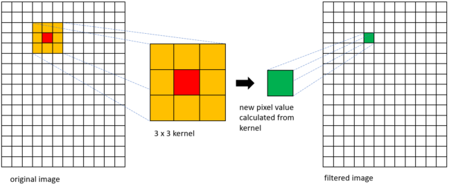
The only differences between the different filters are in the size and shape of the kernel, and in the statistical calculation performed within each kernel. We’ll now look at a suitable filter for each of the types of noise described above.

Mean filtering

The simplest type of filter is just to take the mean of all values in the kernel. Here we assume that each of values in the kernel is equally likely to be near to the true value and so we take a simple average. Obviously, we still need an integer value for the output pixel so this average is rounded to the nearest whole number. The example below shows how the mean output from a 3 x 3 kernel is calculated, and the filtered output from our example image.

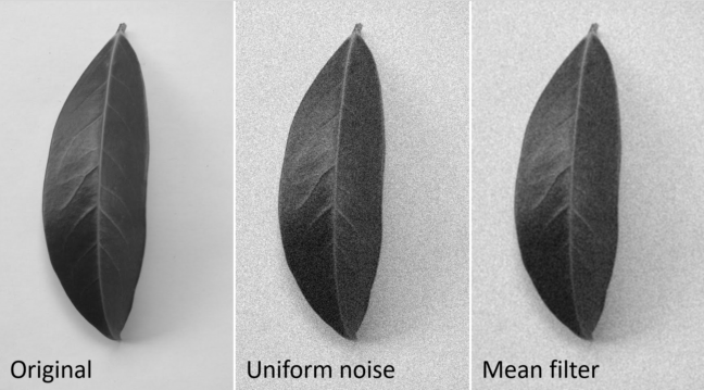
When using a mean filter, since we weight all pixels surrounding the central pixel equally, though noise may be reduced, sharp edges in the image will be smoothed, and the image will become more blurred.

Median filter – salt & pepper noise

In the case of uniform noise, we expect each pixel to be within some margin of error of its true value and use the mean of itself and neighbouring pixels to make a new estimate. This assumes that all the pixels in a small neighbourhood are likely to have similar values, near to the true value we want. This is not the case with salt and pepper noise. Here, isolated pixels will have very high or low values, so just taking a mean will skew the resulting output one way or another, far away from the true value. To ignore the outlying defective pixels then, rather than taking the mean value in the kernel, we instead take the median value.

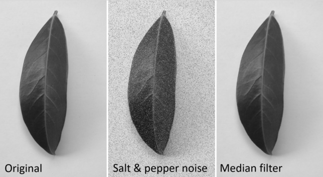
As long as more than half the pixels in any kernel are in the ‘sensible’ range of true values we expect, the median filter does a good job of reducing salt and pepper noise.

Gaussian filtering

Gaussian filtering is the most complicated of the filters we describe in this article to calculate, but in principle it is relatively simple. For Gaussian noise we assume that the measured pixel values are much more likely to take values nearer in intensity to their true values than values further away in intensity from the true value. Similarly, in Gaussian filtering we assume pixels nearer in space to the central pixel of the kernel are more likely to be nearer to the true value than those further way from the centre. To model this, rather than using a simple mean of the kernel, we instead use a weighted mean of values with pixels nearer the centre having greater weights, and those near the edge of the kernel having much lower weights. To calculate the weight (p(x,y)) for each pixel in the kernel we use the following formula:

[p(x,y) = frac{1}{sigma^2 2pi}e^frac{-(x^2+y^2)}{2 sigma^2}]

This process of producing new images by calculating a weighted sum of a pixel and its neighbours in some neighbouring kernel is known as convolution. This technique is of crucial importance in many machine learning approaches to image analysis and computer vision, particularly convolutional neural networks.

Filtering in practice

In practice, when filtering your images, you don’t need to worry about the calculations we have described above. In Fiji, for example, to filter an image you just need to click Process -> Filters, then pick the filter you want to apply to your image. You should recognise Mean, Median and Gaussian Blur from this article. We have explained them here in more detail so you should have a better understanding of what they do, and importantly, what the parameters you can adjust represent. Specifically, for Mean and Median filters, the ‘radius’ parameter is the size of the kernel, while for Gaussian blue the ‘sigma’ parameter refers to the standard deviation used in the Gaussian weights matrix.