Recommended Reading - Mathematical Expression of Climate feedbacks

In this text we show how we can incorporate feedbacks in simple mathematical formulation of climate change and we will go through an example showing how the climate sensitivity due to doubling of CO$_2$ changes as we introduce climate feedbacks.

Applying the concept of radiative forcing ($\triangle Q$), the total change in the surface temperature when the surface temperature is in balance (equilibrium) with the new radiative forcing ($\triangle T_{eq}$) is the direct change in temperature due to the radiative forcing plus the contributions made up by the effect of the radiative forcing ($\triangle Q$) on other climatic parameters ($x_i$) such as snow, ice, humidity etc. that again affect temperature so the total change in near surface temperature will be dependent on the radiatve forcing and changes in other climatic parameters $\triangle T_{eq} = f(\triangle Q, \triangle x_1,.......\triangle x_N)$. We can approximate the total change in near surface temperature as:

$\triangle T _{eq} \approx \frac{dT _{eq}}{d Q} \triangle Q = \frac{\partial T _{eq}}{\partial Q} \triangle Q + \sum_{i=1}^{N} \frac{\partial T _{eq}}{\partial x _i} \frac{\partial x_i}{\partial Q} \triangle Q$

Where the first term on the right hand side is the direct response and the second is the sum of all the feedbacks.

To get some idea of the change in temperature if we have no feedbacks we need to know the response of temperature to the radiative forcing ($dT _{eq} / d Q$). We can do this by consider the change in net radiation at the top of the atmosphere ($R_{toa}$) if we impose a radiative forcing ($dR_{toa}/dQ$). At equilibrium the change in net radiation at the top of the atmosphere given a change in radiative forcing (Q) is zero, using the chain rule we can then write:

$\frac{dR _{toa}}{dQ} = \frac{\partial R _{toa}}{\partial Q} + \frac{\partial R_{toa}}{\partial T_{eq}}\frac{dT_{eq}}{dQ} = 0$

Noting that the direct response $\frac{\partial R _{toa}}{\partial Q}=1$ and rearranging to get $\frac{dT _{s,eq}}{d Q}$ we get

$\frac{dT _{eq}}{dQ} = -\frac{\partial R_{toa}/\partial Q}{\partial R_{toa}/\partial T{eq}} = -\frac{1}{\partial R_{toa}/\partial T_{eq}}$

Thus we need to know the change in the net radiation at the top of the atmosphere due to a change in equilibrium surface temperature ($\partial R_{toa} / \partial T_{eq}$) in order to get the temperature sensitivity to a radiative forcing ($\partial T_{eq} / \partial Q$).

The case of no feedbacks

If temperature is the only climatic parameter that will change the the change in net radiation at the top of the atmosphere due to a change in equilibrium surface temperature is given by Stefan‐Boltzmann’s Law which states that the radiation from a body that absorbs all incoming radiation is depending on the temperature in the $4^{th}$ power.

$E_{BB} = \sigma T_e^4$ ($W/m^2$)

Where $T_e$ is the emission temperature of a blackbody (the temperature the body would have if it absorbed all emission) and $\sigma$ Stefan‐Boltzmann’s constant. If we further assume that the sensitivity of the equilibrium surface temperature to a change in radiative forcing is the same as the sensitivity of the emission temperature ( $\partial T_e / \partial T_{eq} = 1$) we get:

$\frac{T_{eq}}{dQ}=\frac{\partial T_{eq}}{\partial Q} \bigg \rvert _{direct}=-\bigg ( \frac{ \partial R_{toa}}{ \partial T_{eq}} \bigg ) ^{-1} =-\bigg ( \frac{ \partial R_{toa}}{ \partial T_{e}} \frac{ \partial T_{e}}{ \partial T_{eq}} \bigg ) ^{-1} =-\bigg ( \frac{ \partial ( \sigma T_{e}^{4})} { \partial T_{e}} \frac{ \partial T_{e}}{ \partial T_{eq}} \bigg ) ^{-1} =\frac{1}{4\sigma T_{e}^{3}}$

Inserting the emission temperature of the earth‐atmosphere system (255K) we get

$\frac{T_{eq}}{dQ}=\frac{\partial T_{eq}}{\partial Q} \bigg \rvert _{direct}=0.26$ [$K/(W/m^2)$]

In other words, a 1 $W/m^2$ change in radiative forcing will induce a 0.26$^{\circ}C$ equilibrium temperature change.

Including feedbacks

If other variables than temperature are changing the calculation of $\partial R_{toa} / \partial T_{eq}$ is more complicated.

$\frac{T_{eq}}{dQ}=-\frac{1}{\bigg [ \frac{\partial R_{toa}}{\partial T _{eq}} \bigg \rvert _{direct} + \sum_{i=1}^{N} \frac{\partial R_{toa}}{\partial T_{eq}}\bigg \rvert _{x_{i}} \bigg ]}$

Where $x_{i}$ are other climatic parameters such as such as clouds, water vapour, snow, ice etc that again affect temperature.

In the literature the different terms in the denominator are often given as feedback parameters (even if the first term, the direct response, is not a feedback) defined as:

$\lambda_{x_{i}}=-\frac{\partial R_{toa}}{\partial T_{eq}} \bigg \rvert _{x_{i}}$

The unit for the feedback parameters are $W/(m^2K$) and indicate how much the net energy at the top of the atmosphere is changed for a given feedback (in other words how much more or less energy remains in the earth-atmosphere system) for a 1 $^{\circ}C$ change in temperature . Using this notation a negative $\lambda _x$ implies that the feedback is negative and positive values that the feedback is positive. Note that in the literature $\lambda _x$ is sometimes defined without the minus sign. Using the above definition we get:

$\frac{T_{eq}}{dQ}= -\frac{1}{\bigg [ \lambda_{direct} + \sum_{i=1}^{N} \lambda _{x_{i}} \bigg ]}$

Inserting this into equation 1 gives

$\triangle T _{eq} \approx -\frac{1}{\bigg [ \lambda_{direct} + \sum_{i=1}^{N} \lambda_{x_{i}} \bigg ]} \triangle Q$

Thus the temperature change can be approximated by calculating the different feedback parameters. The table below gives typical values for the different feedback parameters.


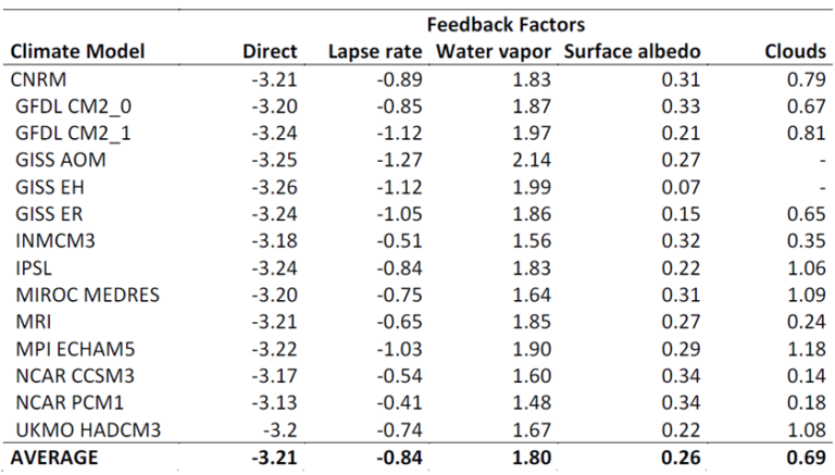
Table: Strength of individual feedback parameters [$W/(m^2K$)] from different state of the art climate models. Values taken from Soden and Held (2006).

Example: Calculating climate sensitivity due to doubling of CO$_2$

From the reading material for week 1 the radiative forcing of CO$_2$ was given as: $RF_{co_{2}} = \alpha ln(C / C_0)$ where $\alpha =5.35, C_o$ is the reference CO$_2$ concentration (usually takes as 280 ppm) and C the CO$_2$ concentration. C and C0 must be given in ppm (parts per million).

A doubling of CO$_2$ then gives a radiative forcing of $3.7 W/m^2$ which together with the average values from the table above we can calculate the temperature change using:

$\triangle T _{eq} \approx -\frac{1}{\bigg [ \lambda_{direct} + \sum_{i=1}^{N} \lambda_{x_{i}} \bigg ]} \triangle Q$

The no feedback result: $\triangle T_{eq} \approx -\frac{3.7}{-3.2} =1.15 ^{\circ}C$

With feedbacks: $\triangle T_{eq} \approx -\frac{3.7}{-3.2 + 1.8 - 0.84 + 0.69 + 0.26} = 2.8^{ \circ }C$