
How to Sort and Filter Data in Excel
Sorting data in Excel
There are many options for sorting data.
You can sort data on common attributes, such as:
- text (A to Z, or Z to A)
- numbers (low to high, or high to low)
- dates and times (newest to oldest, or oldest to newest)
- format (e.g. cell colour).
As well as sorting by individual properties, you can sort data over multiple columns or rows. For example, the following table is initially sorted by ID.
| id | title | season | imdb_rating |
|---|---|---|---|
| 10 | Homer’s Night Out | 1 | 7.4 |
| 12 | Krusty Gets Busted | 1 | 8.3 |
| 14 | Bart Gets an ‘F’ | 2 | 8.2 |
| 17 | Two Cars in Every Garage and Three Eyes on Every Fish | 2 | 8.1 |
| 19 | Dead Putting Society | 2 | 8.0 |
| 35 | Blood Feud | 2 | 8.0 |
| 37 | Mr. Lisa Goes to Washington | 3 | 7.7 |
| 39 | Bart the Murderer | 3 | 8.7 |
| 41 | Like Father, Like Clown | 3 | 7.7 |
| 44 | Saturdays of Thunder | 3 | 7.9 |
But we might want to sort these by season and rating to find the best episodes in each season.
Excel offers additional sorting options, including sorting by custom lists. Custom lists are useful when you want a user-defined order that doesn’t follow existing sort rules. For example, you can’t use an alphabetical sort to sort the values High, Medium, and Low. If you create your own custom list, you can specify the values you want to sort by, in the order you want to sort them.
To sort data in Excel:
- Select a cell in the column you want to sort.
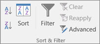
- In the Data tab, go to the Sort & Filter group. Then you have two options.
- To sort values in ascending or descending order based on Excel’s interpretation of the column, click the Sort A to Z or Sort Z to A icons.
- For more sorting options, click the Sort button. You can then specify the Column, what to Sort On, and Order. With the Add Level option, you can perform a secondary level of sorting if needed.
Go to: Sort data in a range or table [1]
Microsoft Support has further instructions and examples of sorting in Excel.
Filtering data in Excel
You can use filters to temporarily hide some of the data in a table, so you can focus on the data you want to see. When filtering, you can specify exact matches or comparisons (‘more than’, ‘less than’) or data that doesn’t match specific criteria. The following comparison operators are available in Excel. You can compare two values by using the following operators. When you use these operators to compare two values, the result is a logical value—it’s either TRUE or FALSE.
| Comparison operator | Meaning | Example | Result (A1=1, B1=2) |
|---|---|---|---|
| = | Equal to | A1=B1 | FALSE |
| > | Greater than | A1>B1 | FALSE |
| < | Less than | A1<B1 | TRUE |
| >= | Greater than or equal to | A1>=B1 | FALSE |
| <= | Less than or equal to | A1<=B1 | TRUE |
| <> | Not equal to | A1<>B1 | TRUE |
To create a filter in Excel:
- Select the data you want to work with.
- Select Data > Filter from the ribbon menu.
- At the top of your selection, select the column header arrow (grey box with downwards arrow).
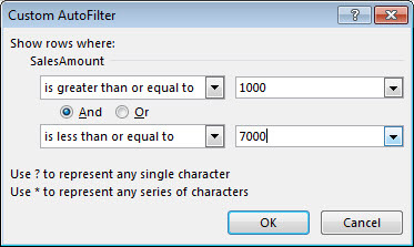
- Select Text Filters or Number Filters, and then select a comparison, such as Between.
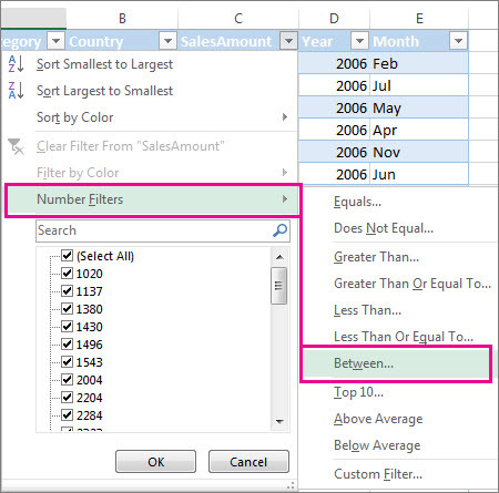
- Enter the filter criteria and select OK.
For more complex filtering you can use logical operators such as AND and OR to select results—depending on which criteria evaluate to true. AND will only evaluate to true if both criteria evaluate to true (e.g. 1<2 AND 3<4). OR evaluates to true if either criteria, or both, evaluate to true (e.g. 1<2 OR 3>4 would evaluate as TRUE).
You can access the Advanced Filter dialog box under Data > Advanced.
Go to: Filter data in a range or table [2]
Go to: Filter by using advanced criteria [3]
These Microsoft Support pages have more examples and instructions about filtering.
Pivot tables
Pivot tables are built into Excel. They allow you to group and summarise large quantities of data quickly and easily. If you have an input table with tens, hundreds, or even thousands of rows, pivot tables allow you to extract answers to a series of basic questions about your data with minimal effort.
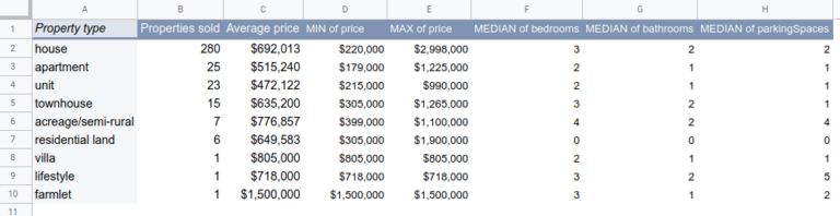
Pivot tables can quickly turn this:
Into:
If you have typical sales data, you can use a pivot table to:
- find the sum of total sales per customer
- count the total number of orders by customer
- find the sum total of sales by item type
- create a summary of sales by customer and item type
- find the average amount of sales to a particular customer in a quarter
- create a summary showing the maximum order value by customer and month
- create a breakout summary of orders by customer, month, and item type.
References
- Sort data in a range or table [Internet]. Microsoft Support. Available from: https://support.microsoft.com/en-us/office/sort-data-in-a-range-or-table-62d0b95d-2a90-4610-a6ae-2e545c4a4654?ui=en-us&rs=en-us&ad=us
- Filter data in a range or table [Internet]. Microsoft Support. Available from: https://support.microsoft.com/en-us/office/filter-data-in-a-range-or-table-01832226-31b5-4568-8806-38c37dcc180e?ui=en-us&rs=en-us&ad=us
- Filter by using advanced criteria [Internet]. Microsoft Support. Available from: https://support.microsoft.com/en-us/office/filter-by-using-advanced-criteria-4c9222fe-8529-4cd7-a898-3f16abdff32b?ui=en-us&rs=en-us&ad=us


Reach your personal and professional goals
Unlock access to hundreds of expert online courses and degrees from top universities and educators to gain accredited qualifications and professional CV-building certificates.
Join over 18 million learners to launch, switch or build upon your career, all at your own pace, across a wide range of topic areas.


